Reducing Quantization Distortion Via Subtractive and Non-subtractive Dithering

Quantizing small amplitude signals can create a correlation between the quantization error and input, leading to significant harmonic components. High-frequency harmonics can alias back to the Nyquist interval onto frequencies that may or may not be a harmonic of the input.

In this article, we’ll see that dithering can suppress both harmonic and non-harmonic spurs. We’ll also take a look at two different types of dithering systems, namely subtractive and non-subtractive topologies, and learn about the important features of each type.

 

High-frequency Harmonics When Quantizing Small Signals

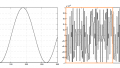
Previously, we discussed that even an ideal analog-to-digital converter (ADC) produces harmonic components when digitizing a low-amplitude signal. For example, by quantifying a 1.11 kHz sinusoid with an amplitude of 0.75 LSB (least significant bit), we get the following waveforms in Figure 1's time domain.

 

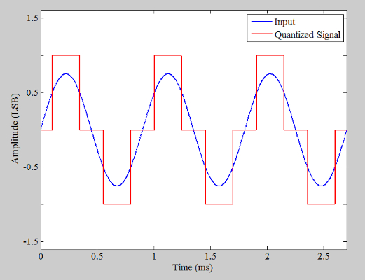
Figure 1. Plot showing the input and quantized signal. 

 

Sampling the quantized signal (the red curve above) at 4 MHz and taking its FFT (fast Fourier transform), we obtain the spectrum below (Figure 2 shows only the DC to 200 kHz range).

 

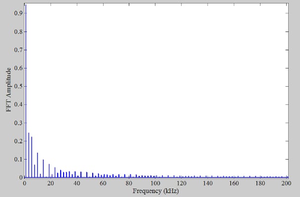
Figure 2. Output spectrum for f_s = 4 MHz.

 

As discussed in the first part of this article, the harmonics in the output spectrum are the artifacts of the quantization operation. By visual inspection, we observe that these harmonics are easily discernible up to about 180 kHz. To produce the above curve, we deliberately use a sampling frequency much higher than that required by Nyquist’s sampling theorem. This high sampling frequency allows us to obtain the true spectrum of the signal without being affected by the limited sampling frequency (as if the signal is an unsampled analog signal).

 

Aliasing Effect Caused by Quantizing Low-amplitude Signals

What if we used a lower sampling rate, say 40 kHz, to acquire the output samples? According to the Nyquist sampling criterion, 40 kHz is large enough to successfully sample and reconstruct a 1.11 kHz sinusoid. However, the square wave-like signal has significant harmonic components up to and beyond 40 kHz. For example, the 33rd and 35th harmonics (at 36.63 kHz and 38.85 kHz) are just below our new sampling frequency f_s = 40 kHz (Figure 3).

 

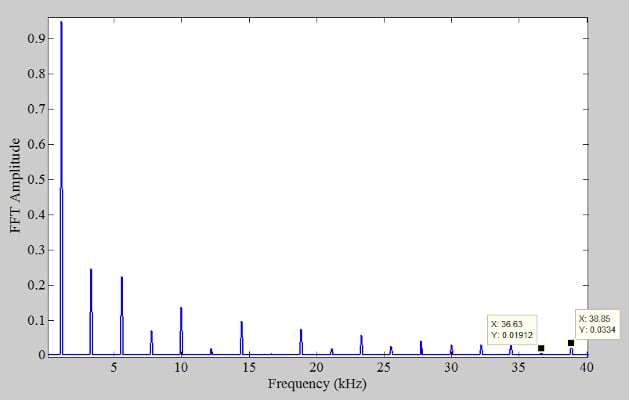
Figure 3. Zoomed-in spectrum for f_s = 4 MHz.

 

Considering the above spectrum, a sampling frequency of 40 kHz doesn’t actually satisfy Nyquist’s sampling condition. As a result, by sampling at 40 kHz, all the harmonics that lie above 20 kHz will be aliased back into the Nyquist interval onto frequencies that may or may not be harmonics of the input. Figure 4 shows the output spectrum for a sampling frequency of 40 kHz.

 

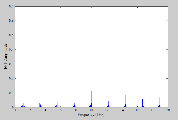
Figure 4. Output spectrum for f_s = 40 kHz.

 

There are harmonic and non-harmonic components in the above spectrum. From Figure 3, we expect the components at 36.63 kHz and 38.85 kHz to alias back onto 3.37 kHz and 1.15 kHz, respectively, when a 40 kHz sampling frequency is used. These aliased components are shown in Figure 5, which provides the zoomed-in version of the output spectrum around the frequencies of interest.

 

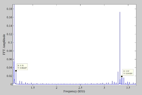
Figure 5. A zoomed-in version of the output spectrum around the frequencies of interest. 

 

Adding dither noise to the signal can break the correlation between the quantization error and input, eliminating the quantization distortion. As a result, we expect the harmonic and non-harmonic components to disappear when a 40 kHz sampling frequency is used along with dithering. To verify this, we add noise with triangular distribution to the input before quantization and then sample it at 40 kHz. The width of the triangular dither PDF (probability density function) is taken to be 2 LSB. In this case, the following output spectrum is obtained (Figure 6).

 

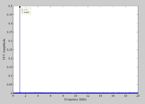
Figure 6. A spectrum of the dithered system for f_s = 40 kHz.

 

With dither applied, there’s only one dominant component at the input frequency. Now that we’re familiar with the functionality of dithering let’s take a look at different methods of applying this technique. 

 

Dithering Methods: Subtractive and Non-subtractive Dithering

These two dithering methods are illustrated in Figure 7.

 

 

Figure 7. A simple breakdown of (a) non-subtractive and (b) subtractive dithering topologies. Image used courtesy of Analog Devices

 

In the subtractive method (Figure 7(b)), the noise introduced to the input is added to the output with opposite polarity, zeroing out the net dithering noise at the system output. With the particular implementation depicted in Figure 7(b), the output of the noise generator is converted to an analog value and subtracted from the input, whereas the digital equivalent of the noise is added to the output through an adder. In the non-subtractive method, the noise is introduced to the input without being subtracted from the output.

As we’ll discuss shortly, subtractive dithering can be more powerful than the non-subtractive version, especially when dealing with quantization distortion. However, in many practical cases, it is not possible to subtract the dither signal from the output simply because the dither noise is not known in the digital domain.

 

Subtractive Dithering—Eliminating Quantization Distortion

The theory behind dithering is relatively complicated and math-intensive. Here, without going through the mathematical details, we’ll take a look at some of the results. As mentioned, we should remember that subtractive dithering is more powerful than the non-subtractive method. For an arbitrary input signal, it can be proven that a subtractive system with appropriate dither noise can render a quantization error that is white, statistically independent of the system input, and has a uniform distribution in the \(-\frac{LSB}{2}\) to \(+\frac{LSB}{2}\) range.

One dither signal that makes the quantization noise have these desired features is white noise with uniform distribution in the \(-\frac{LSB}{2}\) to \(+\frac{LSB}{2}\) range. For a summary of the related mathematical derivations and theorems, you can refer to the book “Design, Modeling and Testing of Data Converters.”

 

Non-subtractive Dithering—Reducing Quantization Distortion

For an arbitrary input, a non-subtractive topology cannot make the total error either uniformly distributed or statistically independent of the input. However, a properly designed non-subtractive system can still considerably improve a quantization system. The simulation results we provided in the first sections of this article correspond to a non-subtractive system. These simulations confirm the effectiveness of a non-subtractive system.

With the proper choice of the dither signal, the power of the total error of a non-subtractive topology P_{Error, Total} can be expressed via Equation 1 (for more details, please refer to the book mentioned in the previous section).

 

\[P_{Error, \text{ } Total}=\frac{LSB^{2}}{12}+\sigma_{v}^{2}\]

Equation 1.

 

The first term in the above equation is the well-known noise power of an ideal quantizer. The second term is the variance of the dither noise. Equation 1 intuitively makes sense as it shows that the dither noise power is added to the quantization noise power, determining the noise floor of the whole system. If we use a dither noise with a larger variance, the output noise level will increase. In other words, by adding the dither noise to the input, we are trying to break the correlation between the quantization noise and input at the expense of slightly raising the noise floor. 

 

Common Dither Signals

One important feature of the dither signal is its probability density function. Dither signals with Gaussian, rectangular, or triangular distribution are used for different applications. The rectangular and triangular dither signals that can be used to reduce the quantization distortion of a non-subtractive system are shown in Figure 9.

 

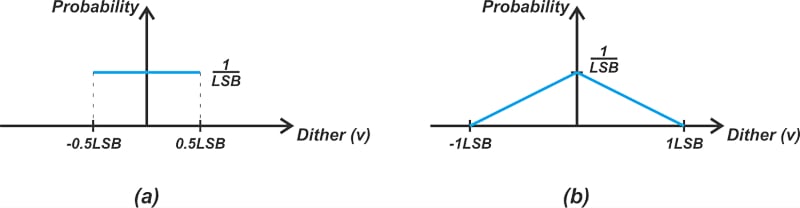
Figure 9. Diagrams of (a) rectangular and (b) triangular dither signals for eliminating quantization distortion.

 

The variance of the above rectangular and triangular dither signals is \(\frac{LSB^{2}}{12}\) and \(\frac{LSB^{2}}{6}\), respectively.

For a Gaussian dither, the recommended variance is \(\frac{LSB^{2}}{4}\).

By substituting these values in Equation 1, we can calculate the increase in the noise floor for different dither types. Compared with an undithered system, applying rectangular, triangular, and Gaussian dithers can increase the noise floor of a non-subtractive system by 3 dB, 4.8 dB, and 6 dB, respectively.

For more information, please refer to the book “Introduction to Signal Processing” by S. J. Orfanidis. As a side note, Dr. Orfanidis has generously made his book available for free. This well-written book has been one of the main references for my two-part series.

 

---

 

To see a complete list of my articles, please visit this page.