Technical Article

The Small-Signal Open-Loop Transfer Function of the Moog Filter

August 02, 2019 by Sam Gallagher

We are analyzing the behavior of the Moog ladder filter. In this section, we will analyze the heart of the topology and express the small-signal open-loop transfer function of the filter as a whole.

Voltage-controlled filters (VCFs) were a mainstay of the analog synthesizer. But one filter stands above the rest, for being creative, effective, and (I have on good authority) audibly "brilliant": the Moog ladder filter.

In this series, we’re analyzing the behavior of the Moog ladder filter, starting with a small-signal open-loop analysis.

In the previous article, we went over the primary elements of the filter and analyzed the driver section. Now, we will analyze the heart of the topology (the filter sections) and express the small-signal open-loop transfer function of the filter as a whole.

In part 1, we saw the full schematic of the Moog ladder filter and reduced it to the form shown in Figure 1.

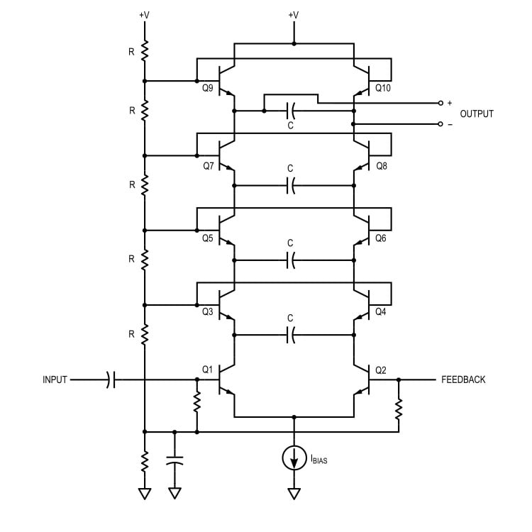
Figure 1. The Moog filter

We divided the topology into three elements:

A driver stage
An intermediate filter stage
An output filter stage

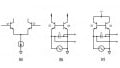
The three stages are shown in Figure 2.

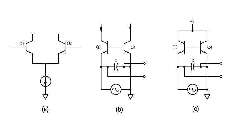
Figure 2. The three elements of the ladder filter topology. (a) The driving differential pair. (b) A mid-ladder low-pass filter section. (c) The top-most output filter section.

Also in part 1, we derived a relationship between the voltages and currents in the driver stage, seen above in Figure 2(a). Now, we’ll analyze the filter stages depicted in Figures 2(b) and 2(c).

The Individual Filters of the Moog Filter

The filter sections are similar to one-another, except that one is driving another stage in the ladder, while the other is tied to the supply. The same mechanism is at work in both of them, so we will only analyze the one shown in Figure 3.

Figure 3. One filter section in the Moog filter, with a differential driving current.

For small-signal analysis, we can make the following simplifications, shown in Figures 4, 5, 6, and 7.

Figure 4. Using the fact that the bases are held at constant potential and leaving the capacitor as a reactance.

Figure 5. Removing the shorted transistor.

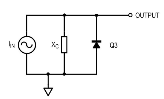
Figure 6. The transistor Q3 is connected in a diode configuration, so we can replace it schematically with a diode.

The circuit in Figure 7 may not, at first glance, look like a filter.

Figure 7. The diode/transistor is finally replaced with a hybrid-pi model.

This is fair—it's not common to see a current-driven RC circuit like this. But, noting that the two parallel components act as a current divider instead of a voltage divider, it begins to make sense.

As the capacitive reactance X_c decreases (with increasing frequency), the voltage across the capacitor decreases.

The output voltage of this circuit is the voltage across the capacitor, and describing the transfer function as a transimpedance r_tr, we find that:

$$ r_{tr} = \frac{v_{out}}{i_{in}} = \frac{-1}{2j \omega C + g_m} $$

Where

$$g_m = \frac{I_C}{V_T}$$

For transistor bias (drive) current I_C, and we assumed high beta.

For intermediate filter stages, the output current—g_mv_out—becomes the input current to the next section. This current is:

$$ i_{out} = i_{in} \frac{-g_m}{2j\omega C + g_m} $$

Which is the only other result we'll need to calculate open-loop gain.

To summarize this filter section: We have shown that the input current causes a voltage drop across the capacitor which is proportional to the capacitive reactance. As the frequency increases, the voltage decreases, giving us our low-pass action. It's like a current-driven RC filter between the capacitor and the transistor equivalent base impedance (the transconductance). For the intermediate stages, the transistor currents are used as input currents to the following section, while the capacitor voltage itself is taken as the output of the top-most stage.

Putting It All Together: Calculating Open-Loop Gain

We've described the transfer functions of the driver and filter sections. Now we are prepared to calculate open-loop gain. For n filter stages, we can combine our previous results (a driver, n-1 mid-ladder filter sections, and an output filter section), and find, taking the left side of the output capacitor as positive:

$$ v_{out} = \left ({g_m v_{in}}\right ) \left ( \frac{-g_m}{2j\omega C + g_m} \right )^{n-1} \left ( \frac{-1}{2j\omega C + g_m} \right ) $$

Which simplifies to:

$$ v_{out} = \pm v_{in} \left ( \frac{g_m}{2j\omega C + g_m} \right )^{n} $$

Where $$v_{out}$$ is positive for n even, and negative for n odd. The open-loop voltage gain is:

$$ A = \pm \left ( \frac{g_m}{2j\omega C + g_m} \right )^{n} $$

Using the fact that $$g_{m}$$ is approximately equal to $$\frac{1}{{r_e} '}$$, we can rewrite this is a more familiar form,

$$ A = \pm \left ( \frac{1}{j\omega r_e’C + 1}\right )^n $$

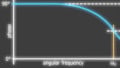
Which, you may notice, strongly resembles the transfer function of an RC low-pass filter,

$$ A = \frac{1}{j\omega RC - 1} $$

And we’ll talk more about this in the next article.

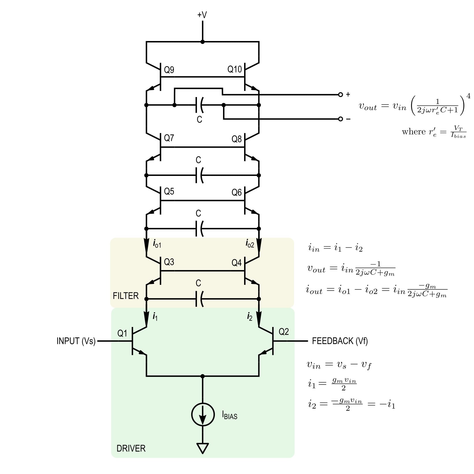
Figure 8. Summary of the Moog ladder filter behavior. Click to enlarge.

We can summarize the behavior of the Moog filter as follows (see Figure 8): The bias current sets the quiescent point of the transistors and this current is shared between both sides of the ladder.

Neglecting feedback, an input voltage on the left side drives a small-signal current through the branches. A differential signal between the branches creates a potential difference across the capacitors, allowing "filtering" to occur. One way to look at this is that the transimpedance of the transistors creates an RC filter with the capacitors.

The output, taken as the potential across the top-most capacitor, is dependent on the small-signal current flowing through that capacitor.

To this point, we've assumed a few important things:

All transistors share the same beta (i.e., they are all matched).
The current through the base of each transistor is negligible.
The transistors act as ideal dependent current sources (no Early effect).
All transistors are biased in the active region.
The driver stage common-mode voltage is negligible.
The bias current source is ideal.

Even with these idealizations, the circuit suffers from temperature dependence (hidden in the g_m terms and transistor betas). However, recall that this circuit was used in analog synthesizers and these imperfections are considered to give the filter "character".

Conclusion

In this second part of our analysis, we have investigated the small-signal behavior of the famous Moog ladder filter. We made some important assumptions and idealizations to simplify analysis and arrived at a general transfer function for an n-stage filter.

Going forward, we'll extend our analysis by considering feedback, and analyze the filter sections in more detail to understand the filter parameters. The Moog ladder filter has also inspired some copy-cat designs, and we will take a look at those as well.

As far as I am aware, this is the first Moog filter analysis that has been published for the general reader, and I'm delighted to be the one to introduce designers to this creative and intelligent design.