 Facebook
 Google
 GitHub
 Linkedin
Understanding Current-Voltage Curves
This article discusses I-V curves for passive components, voltage sources, and current sources.
This article discusses I-V curves for passive components, voltage sources, and current sources.
The current (I) - voltage (V) relationship of electrical components can often provide insight into how electronic devices are used. More specifically, many non-linear devices such as diodes and transistors are used in operating regions in which they behave like ideal components—such as current sources, voltage regulators, and resistors.
An understanding of I-V curves often provides insight into knowing how the device operates and helps us know how to operate a device in a way that enables the required functionality.
We'll begin by looking at how to obtain an I-V curve for any component.
Obtaining I-V Curves
Method 1: Voltage Sweeps
The current-voltage (I-V) relationship for a device is a current measured for a given voltage. For devices that do not supply power, I-V curves are obtained by using linear voltage sweeps. Voltage sweeps involve the linear variation of the voltage, to obtain the corresponding measured output current. Because it is impossible to physically sweep through all the voltages in an instant, it is important to understand that these measurements are made with respect to time as well.
Figure 1.1 illustrates the translation of voltage sweep with respect to time (V vs t) onto the X-axis of the current-voltage graph (I vs V). It is important to understand that the V vs t information is implicitly present in the I vs V curve. The notion of time is relevant for components that respond to a change in voltage (such as a capacitor) rather than the instantaneous voltage (as with a resistor).
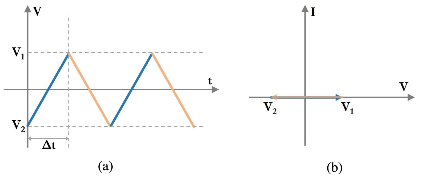
Figure 1.1 (a): A linear sweep of voltage (V) with respect to time (t); (b): the corresponding voltage sweep in the current (I) - voltage (V) curve.
If you have a device that supplies voltage or current, such as a battery or a solar panel or a regular power supply, you cannot change the voltage across the device, because there is a specific voltage or current being generated by the device. For these devices, I-V curves are obtained by load switching.
Method 2: Load Switching
Load switching is a method that involves measuring the current supplied by the power source for varying load resistance. The load is the device that electrical power is being delivered to, where power is defined as $$P = V \times I$$.
Typically, a resistor is used as the load to measure the power delivered by a current or a voltage source because they are linear devices that do not exhibit properties of hysteresis, i.e., the operation of the resistor does not depend on its previous state. Because devices can operate with small values of resistance (1-10Ω) as well as large values of resistance (10-1000kΩ), the resistors are varied logarithmically, i.e., from 10 to 100 to 1000 and so on.
The current that is supplied by the power supply is measured by an ammeter for each value of load resistance—shown in Figure 1.2(b)—and the voltage across the load is measured using a voltmeter—shown in Figure 1.2(c).
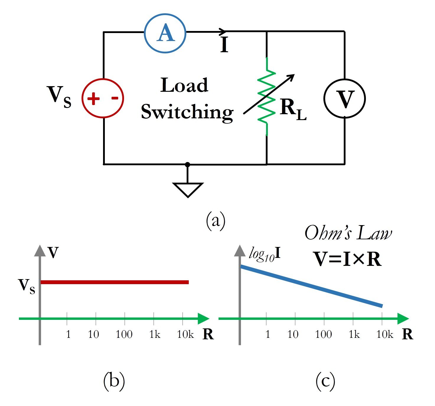
Figure 1.2 (a) Schematic circuit for load switching I-V curve measurements; shown here is an example of an ideal voltage source. The value of RL is varied over a large range and for each value of resistance the voltage (b) and current (c) are measured.
Note that in Figure 1.2(c), the (base 10) logarithmic value of current decreases linearly. This is because a resistor is governed by Ohm's law, and this is an ideal voltage source at a fixed voltage VS; as the resistance value increases logarithmically, the current value decreases logarithmically. Load switching techniques are used to measure the I-V characteristics of devices and circuits that supply power, such as voltage regulator circuits, solar cells, and batteries.
I-V Curves of Ideal Components
Using linear voltage sweeps and load switching, we will now look at the I-V curves of ideal components. In general, if the device requires power to operate, the voltage sweep method is used.
On the other hand, if the device acts as a source of power, the load switching method is used. Based on their basic definitions, we can derive the I-V curves of ideal passive components (resistors, capacitors, and inductors) using the concept of linear voltage sweeps. We will use the concept of load switching for the I-V curves of an ideal voltage source and an ideal current source.
Ideal Resistor
Let's start with one of the more familiar ideal components: the resistor.
The resistor is a component that represents a linear relationship between voltage and current as dictated by Ohm's law, i.e., $$V=I \times R$$. The graphical representation on the I-V curve of the Ohm's law equation is a straight line passing through the origin, as shown in Figure 2.
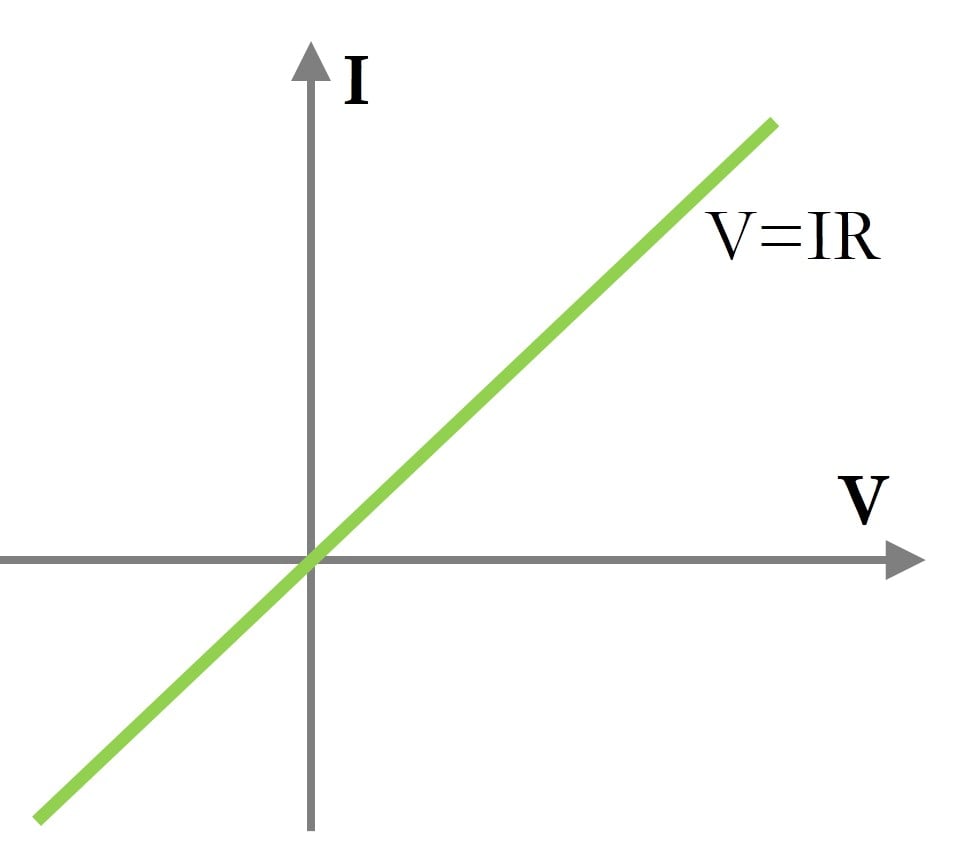
Figure 2. The I-V curve of an ideal resistor is a straight line that passes through the origin.
Ideal Voltage Source
An ideal voltage source is a component that can provide a fixed voltage regardless of the current delivered to the load.
For example, let's say a voltage source supplying 10V is connected across a resistor. If the value of the resistor is $$10k\Omega$$, then the current drawn by the resistor from the voltage supply will be dictated by Ohm's law, which is $$ I = \frac{V}{R} = \frac{10V}{10k\Omega} = 1mA$$. If the value of the resistor is 1Ω, then the current drawn will be 10A!
A real voltage supply is limited with respect to the amount of current it can supply for a given voltage, but an ideal voltage source is not. Therefore, the I-V curve for an ideal voltage supply will be a straight line parallel to the Y-axis (see Figure 3). An empirical I-V curve for a real voltage source would be obtained using the load-switching method.
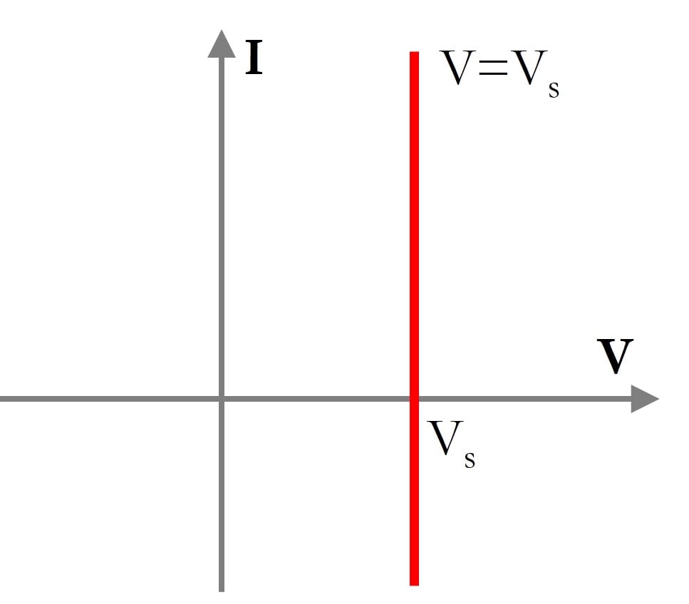
Figure 3. The I-V curve of an ideal voltage source is a straight line parallel to the current (I) axis—i.e., regardless of the current passing through the device, the voltage will not change.
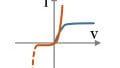
The Zener diode is a non-linear, passive device that is used as a voltage regulator when it is operated in reverse bias. The (idealized) I-V curve of a reverse-biased Zener diode shows that it stays at a particular voltage (determined by the manufacturing process) regardless of the current passing through it. We will be looking at the I-V curve of a Zener diode in a future article.
Ideal Current Source
An ideal current source is a component that can provide a fixed current regardless of the voltage across the component, itself. In other words, a 5A ideal current source would deliver exactly 5A to a 1Ω load resistor or to a 1 kΩ resistor, even though the second resistor would generate a voltage drop of 5000V! This is highly impractical but, nonetheless, ideal current sources are useful tools in circuit analysis.
The I-V curve for an ideal current source is a straight line parallel to the X-axis (see Figure 4). An empirical I-V curve for a real current source would be obtained using the load-switching method.
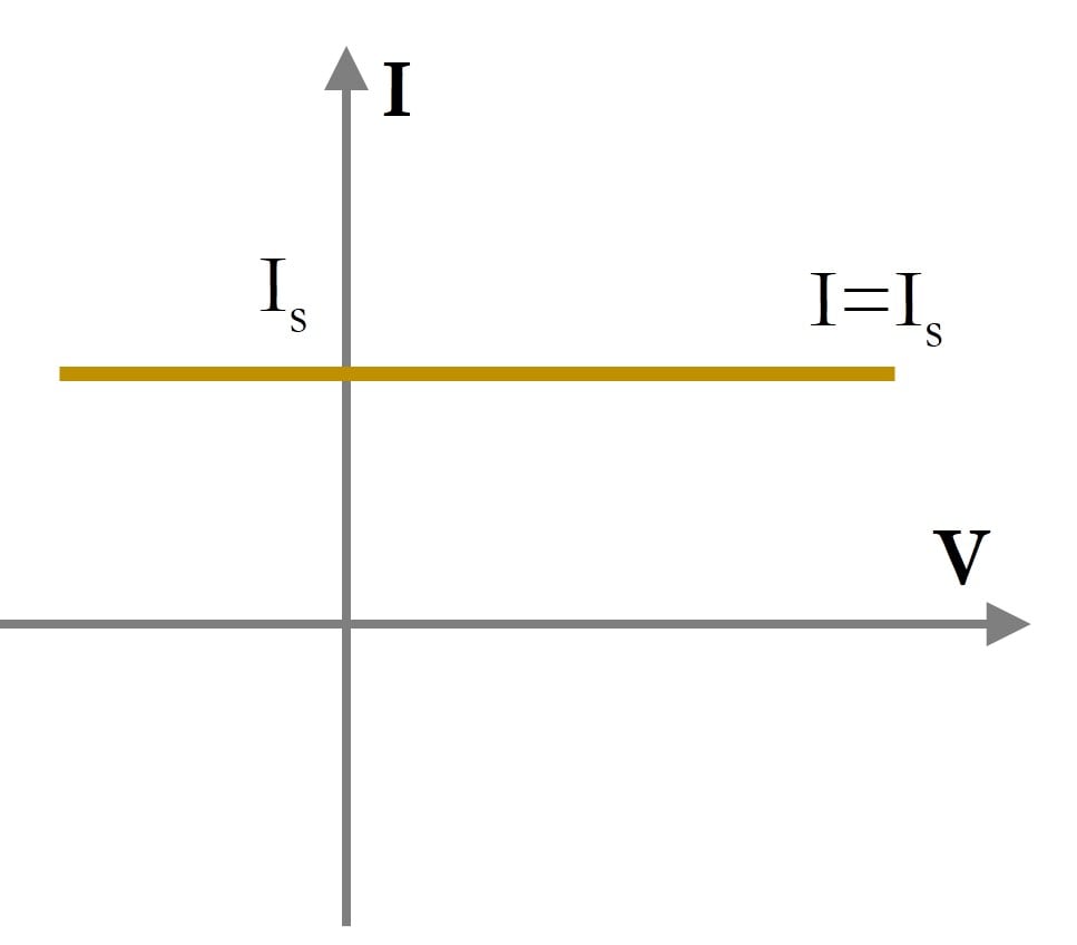
Figure 4. The I-V curve of an ideal current source is a straight line parallel to the voltage axis; i.e., the current flowing from the source is the same regardless of the voltage across it.
Though "current supplies" are not nearly as common as voltage supplies, many analog transistor circuits are biased using a constant-current source. Also, a MOSFET operating in the saturation region exhibits behavior similar to that of a (voltage-controlled) current source.
Ideal Capacitor
In a resistor, the voltage is determined by the resistance and the current flowing through the resistor. Capacitors and inductors are fundamentally different in that their current-voltage relationships involve the rate of change. In the case of a capacitor, the current through the capacitor at any given moment is the product of capacitance and the rate of change (i.e., the derivative with respect to time) of the voltage across the capacitor.
$$I=C\cdot\frac{\text{d}V}{\text{d}t} $$
Because we are using a linear voltage sweep, the current through the capacitor is constant when the voltage is increasing or decreasing. When the voltage changes from a positive slope (shown in blue in Figure 5) to a negative slope (orange), the direction of the current reverses; this is represented in the current vs. time plot as a change from the positive-current section of the graph to the negative-current section of the graph.
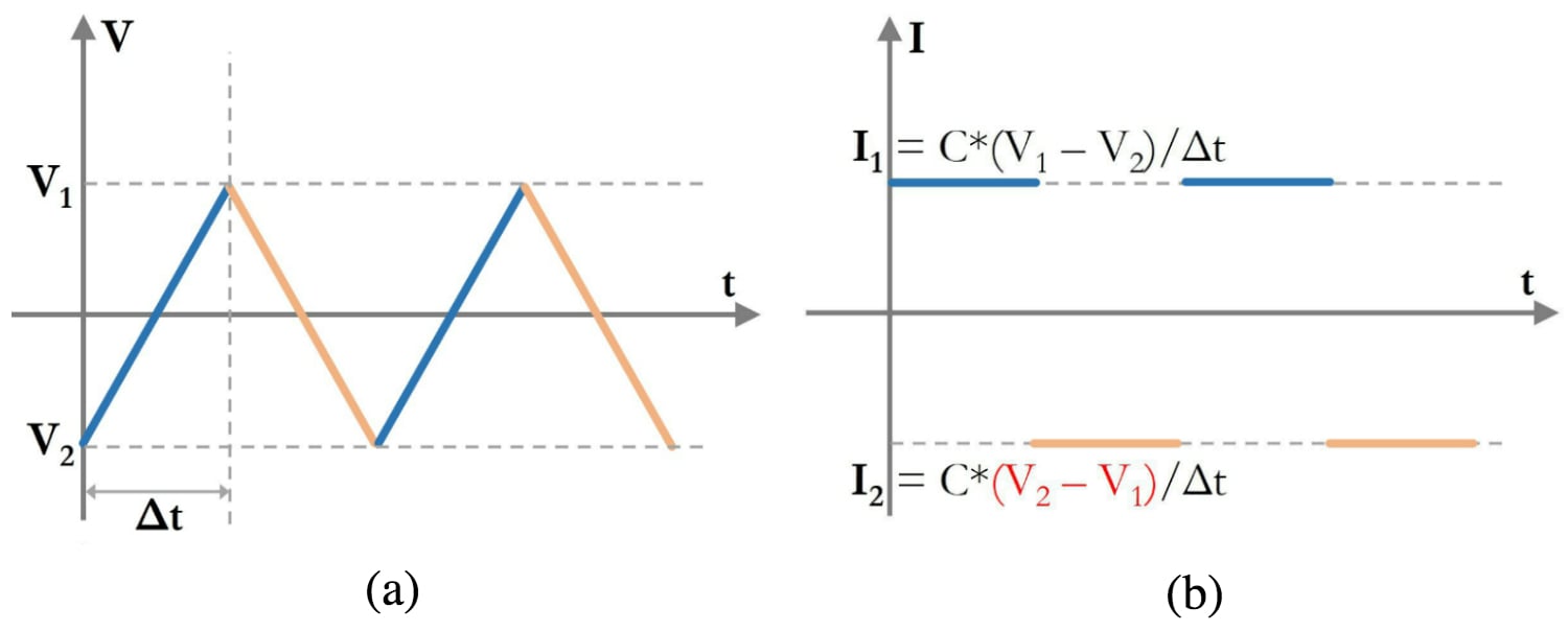
Figure 5 (a) Linear voltage sweep and (b) the corresponding capacitor current vs. time.
The I-V relationship of an ideal capacitor is shown in Figure 6. The magnitude of the current is constant, but two horizontal lines are needed because the direction of the current changes depending on whether the voltage is moving from V1 to V2 or V2 to V1. When the voltage has a positive rate of change, the current is positive (indicated by the blue arrowhead); when the voltage has a negative rate of change, the current is negative (indicated by the orange arrowhead).
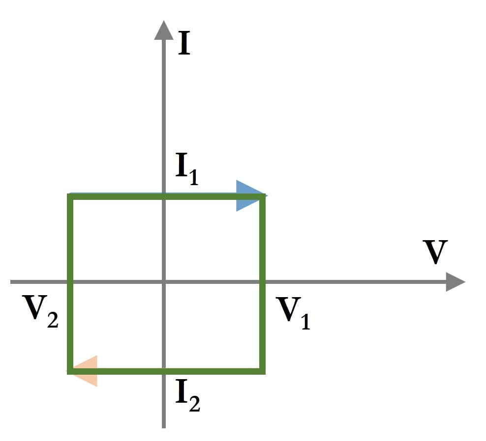
Figure 6. I-V curve for an ideal capacitor based on the voltage sweep shown in Figure 5.
Ideal Inductor
The voltage across an inductor is the product of inductance and the rate of change of the current flowing through the inductor:
$$V=L\cdot\frac{\text{d}I}{\text{d}t} $$
This means that the current is proportional to the integral of voltage, and this is what we see in the following plots. The current increases in magnitude as the (negative) area under the voltage curve increases. But when the voltage crosses the time axis, the positive area under the curve starts to balance out the negative area under the curve, and this causes the current magnitude to decrease toward zero.
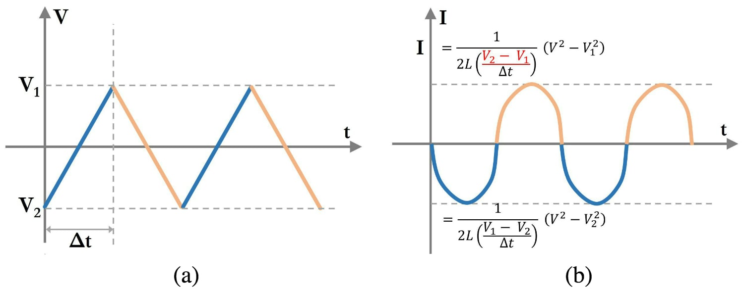
Figure 7 (a) Linear voltage sweep and (b) the corresponding inductor current vs. time.
Note the difference between the capacitor and the inductor: With a capacitor, current is proportional to the derivative of voltage, and thus a linear voltage sweep translates to constant current. With an inductor, current is proportional to the integral of voltage, and thus a linear voltage sweep translates to a quadratic shape in the current vs. time plot.
The I-V relationship of an ideal inductor is shown in Figure 8. The magnitude of the current gradually increases and then decreases as the voltage moves from V2 to V1 or from V1 to V2. The direction of the current is negative as the voltage moves from V1 to V2 and positive as the voltage moves from V2 to V1.
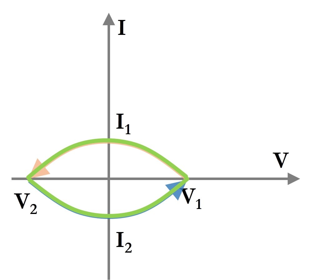
Figure 8. I-V curve for an ideal inductor based on the voltage sweep shown in Figure 7.
Summary
The table below summarizes some of the insights we have obtained by looking at the I-V curves of several ideal devices. In a future article, we will look at I-V curves of non-linear devices.
| Device | Requires Power? | I-V Method | Description of the Graph | Passes Through Origin? |
| Ideal Resistor | Yes | Voltage Sweep | Straight line passing through origin | Yes |
| Ideal Voltage Source | No | Load Switching | Straight line parallel to current axis | No |
| Ideal Current Source | No | Load Switching | Straight line parallel to voltage axis | No |
| Ideal Capacitor | Yes | Voltage Sweep | Closed rectangle around origin | No |
| Ideal Inductor | Yes | Voltage Sweep | Closed parabolic loop around origin | No |
Related Content


I love this site. Please keep writing these amazing articles, they very informative and useful. I like how this site goes all over the picture, from basics to advanced electronics to cover as much material as possible. Keep up the good work.
Thanks for the article. If I understand correctly in Figure 8. I1 should be negative and I2 positive. Also according to my calculation in Figure 7. Imin should be (1/(2L*(V1-V2)/∆t))*V1^2 and Imax should be (1/(2L*(V2-V1)/∆t))*V2^2 . Could you please clarify this?