 Facebook
 Google
 GitHub
 Linkedin
Understanding Phase-Locked Loop Transient Response
In this article we’ll use SPICE simulations to take a close look at how a phase-locked loop enters the locked state.
In this article we’ll use SPICE simulations to take a close look at how a phase-locked loop enters the locked state.
So far I’ve written two articles on phase-locked loops (PLLs). The first was a general introduction to phase-locked loops, and the second presented and explained an LTspice circuit that can be used as a platform for PLL experimentation.
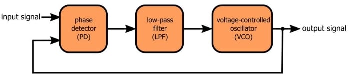
In this article we’ll use SPICE simulations to more thoroughly understand PLL transient behavior. Just in case you need a reminder, here is the structure of a very basic PLL.
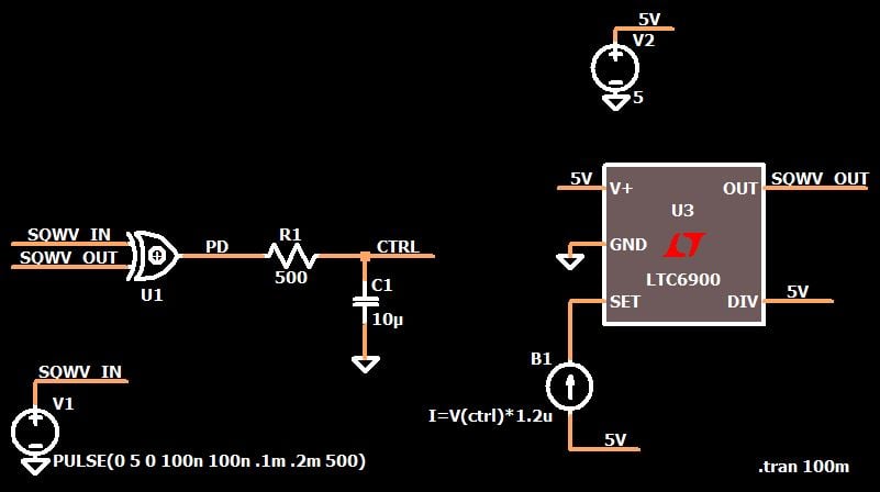
And here is the LTspice circuit, so you don’t have to click back to the previous article.
In my experience, negative-feedback systems in general can be difficult to analyze qualitatively. PLLs are especially difficult, and I think that this is partially due to the fact that the control variable is transformed as it travels through the loop.
In a non-inverting op-amp configuration, for example, the input is a voltage, the output is a voltage, and the feedback appears as a voltage at the op-amp’s inverting input terminal. In a PLL, the situation is very different. The input variable is a phase (or a frequency, depending on your perspective) and the feedback variable is a phase (or a frequency), but in between these two stages the variable is a voltage amplitude. (After thinking about this a bit more, I’m wondering if this characteristic is a greater impediment to quantitative analysis than to qualitative analysis).
Another confusing aspect of PLL functionality is the nebulous relationship between frequency and phase. The VCO generates a frequency, but its frequency variations are used to establish a phase relationship, and this fixed phase relationship results in identical input and output frequencies, through the action of a phase detector. The two fundamental points that you need to keep in mind if you expect to unravel this mystery are the following:
- Frequency variations can be used to establish a phase relationship. Imagine randomly varying the frequency of one square wave until the rising edge happens to coincide with the rising edge of another square wave. You now have phase alignment (but the alignment won’t last if the frequencies are different).
- The output of a phase detector can be constant only when the input frequencies are exactly equal (because frequency differences will always lead to gradual variations in the phase alignment of the two signals). Thus, a PLL-style feedback system that causes the output of the phase detector to settle on a constant value will force the output frequency to be identical to the input frequency.
Finding Frequency...and Phase
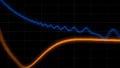
I concluded the previous article with a plot of control voltage (i.e., the low-pass-filtered phase-detector signal) versus time. Let’s look at this response again.
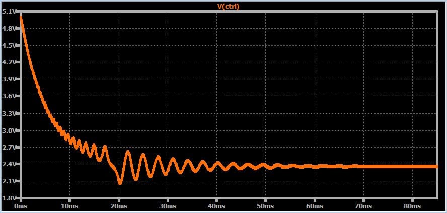
This is a very interesting plot, in my opinion. The initial conditions result in a control voltage that begins at the upper end of its 0–5 V range. Next, the voltage quickly decreases until it is in the general vicinity of the steady-state value (~2.36 V). It then experiences some high-amplitude oscillations before beginning to settle on the final value.
Stage 1
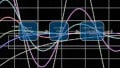
The frequencies are initially completely different (as expected). The output waveform is ~10.5 kHz, compared to the fixed 5 kHz frequency of the input signal:

As you can see from the phase-detector output, though, this frequency difference doesn’t result in anything near 100% duty cycle.

Consequently, the control voltage makes a dive toward the average value of the PD output. During this first stage, the system isn’t really searching for the steady-state condition. It’s more a preparation for the searching phase.
Stage 2
By the 10 ms mark, the frequencies are much closer (6 kHz vs. 5 kHz):

This smaller difference in frequency results in the lower-frequency control-voltage variations that become prominent during the 10–19 ms portion of the plot.
I’m sure that you’ve already noticed the discontinuity that occurs at ~19 ms: there is a clear interruption in the regularity of the oscillations. Perhaps you also observed that this discontinuity coincides with the first time that the control voltage reaches the value on which the output will eventually settle (i.e., once it has achieved lock).
I’m not sure exactly how to interpret this event, but it seems to initiate the third stage of the transient response: the system has found the steady-state value, which initially is the DC offset of the oscillations and gradually becomes the voltage amplitude itself as the oscillations die away.
Stage 3
During stage 3, the control voltage oscillates as the system attempts to reach the state in which 1) input and output frequencies are identical and 2) the proper input–output phase relationship has been established. Remember that the PLL cannot reach a steady state until both of these conditions have been fulfilled. This process makes me think of a person rotating a frequency knob back and forth—watching the scope, trying to reach and maintain a specified phase relationship, rotating less and less as the phase relationship tends to stay closer to the desired value.
This next plot demonstrates the result of all this searching and adjusting and low-pass filtering and negative feeding-back. The frequencies are identical, and the phase difference is exactly what the phase detector needs to produce the average value that holds the VCO at the correct frequency.

Conclusion
In this article we used SPICE simulations to gain some insight into the process by which a phase-locked loop reaches the locked state. It is interesting to see how the transient response exhibits the same oscillatory settling behavior that we expect from other types of control systems, despite the fact that PLLs are quite different from feedback circuits such as op-amp-based amplifiers. In the next article we’ll modify the low-pass filter and observe how these changes influence the PLL’s performance.
Feel free to download my LTspice schematic by clicking on the orange button.


why ((The initial conditions result in a control voltage that begins at the upper end of its 0–5 V range))?