Facebook
 Google
 GitHub
 Linkedin
Achieving Faster Composite Op-Amp Dynamics by Expanding the Frequency Bandwidth
This is Part 3 of the series of articles about composite amplifiers. In this section, we are going to show how to achieve faster op-amp dynamics by expanding the frequency bandwidth.
In Parts 1 and 2 of a three-article series on composite amplifiers, we have investigated how to boost the output current drive capability of an op-amp and simulate our example voltage buffer in PSpice.
Now, we are going to show how to achieve faster op-amp dynamics by expanding the frequency bandwidth.
Expanding the Frequency Bandwidth
The open-loop gain of most op-amps exhibits a constant gain-bandwidth product (constant GBP). The most salient consequence of this constancy is the fact that the higher the noise gain of an op-amp circuit is, the lower the closed-loop bandwidth. For instance, if we configure the op-amp as a noninverting amplifier, in which case the noise gain coincides with the closed-loop gain A, then the closed-loop bandwidth is
\[f_B = \frac {GBP}{A}\]
Equation 1
So, if we use an op-amp with GBP = 1 MHz and configure it for a noninverting gain of A = 10 V/V, then we get fB = 106/10 = 100 kHz. For A = 100 V/V we get fB = 10 kHz, and for A = 1,000 V/V we get fB = 1 kHz.
What if we wanted to use this op-amp as an audio preamplifier with a gain of 1,000 V/V and a bandwidth of fB = 20 kHz, which represents the upper limit of the audio range?
Clearly, a single 1-MHz op-amp won’t do it, so let’s see if we can enlist the help of a second, similar op-amp to raise fB from 1 kHz to 20 kHz. Figure 1 shows a popular realization of this concept.
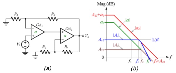
Figure 1. (a) Composite amplifier to achieve a wider bandwidth. (b) Straight-line Bode plots
In the figure, you can see (a) a composite amplifier to achieve a wider bandwidth. and (b) straight-line Bode plots where:
- |a| is the open-loop gain of each op-amp, and ft is the transition frequency (ft = GBP in the present rendition)
- |ac| is the composite amplifier’s open-loop gain
- |A2| is the closed-loop gain of OA2, and f2 is its –3-dB frequency
- |Ac| is the composite amplifier’s closed-loop gain, and fc is its –3-dB frequency
- |β| is the feedback factor around the composite amplifier
- a0, Ac0, and A20 identify the DC values of the above gains
Here, OA1 is the primary op-amp and OA2 is the secondary op-amp, both having an open-loop gain of a. OA2 is configured as a noninverting amplifier with a closed-loop gain of A2 with a DC value of
\[A_{20} = 1 + \frac {R_4}{R_3}\]
Equation 2
By Equation 1, with GBP replaced by ft, the closed-loop bandwidth of OA2 is
\[f_{2} = \frac {f_t}{A_{20}}\]
Equation 3
Together, OA1 and OA2 form a composite amplifier with an open-loop gain of
\[a_{c} = a \times A_2\]
Equation 4
The presence of OA2 inside OA1’s feedback loop has two effects:
- It expands the open-loop gain from a to ac. Due to the logarithmic nature of decibels (the log of a product equals the sum of the logs), the DC values a0 and A20 add up in the manner shown.
- It establishes a pole frequency at f2, which causes the slope of the |ac| curve to change from –20 dB/dec to –40 dB/dec, as shown. This pole frequency will erode the phase margin of the loop around OA1, so we must be vigilant that the overall circuit does not get destabilized.
The composite amplifier of Figure 1(a) is in turn configured as a noninverting amplifier with a feedback factor of β = R1/(R1 + R2). The reciprocal 1/β is called the noise gain, and
\[\frac {1}{\beta} = 1 + \frac {R_2}{R_1}\]
Equation 5
(Recall that for a noninverting op-amp the noise gain and the closed-loop gain coincide, so Ac0 = 1/β). Were OA1 operating alone, its closed-loop bandwidth would be f1 (see Figure 1(b)).
However, the presence of OA2 expands the closed-loop bandwidth from f1 to fc, where fc is the crossover frequency of the |ac| and |1/β| curves. It is precisely this bandwidth expansion that we wish to exploit.
To gain better insight, consider the PSpice circuit of Figure 2, simulating a composite amplifier with a closed-loop gain of 1,000 V/V, or 60 dB.
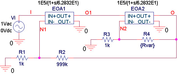
Figure 2. PSpice circuit for a composite amplifier using Laplace blocks to simulate 1-MHz op-amps.
Figure 3(a) shows the effect of stepping EOA2’s closed-loop gain |A2| in 10-dB increments via R4. For |A2| = 0 dB things go as if EOA1 were operating alone, giving a closed-loop DC gain of 1,000 V/V (= 60 dB) with a closed-loop bandwidth of 1 kHz.
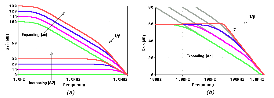
Figure 3. Visualizing the effect of 10-dB increments in EOA2’s closed-loop gain |A2| in the circuit of Figure 2. Effect on the composite amplifier’s (a) open-loop gain |ac|, and (b) closed-loop gain |Ac|.
Increasing |A2| expands the composite amplifier’s open-loop gain |ac| along both the vertical and the horizontal axes, while at the same time reducing EOA2’s closed-loop bandwidth f2, as per Equation 3.
Figure 3(b) shows the effect on the composite amplifier’s closed-loop gain Ac: all curves exhibit the same DC value of 60 dB; however, the bandwidth increases with |A2|.
It is interesting to observe, in Figure 4(a), how OA1 and OA2 cooperate, in complementary fashion, to maintain a constant DC value of 60 dB.
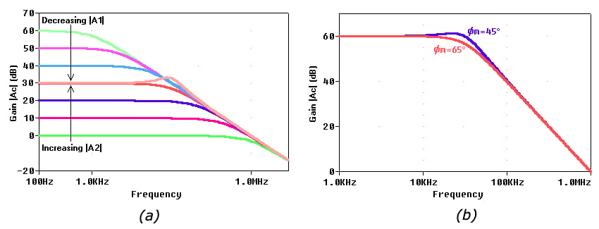
Figure 4. Visualizing the effect of 10-dB increments in EOA2’s closed-loop gain |A2| upon EOA1’s closed-loop gain |A1| in the circuit of Figure 2 (b). The composite amplifier’s closed-loop gain |Ac| for phase margins of 45° and 65°.
As |A2| rises, |A1| drops in such a way that their DC values keep adding up to 60 dB as 0 + 60, or 10 + 50, or 20 + 40, or 30 + 30. However, also OA2’s pole frequency f2 drops, and in so doing it gradually erodes OA1’s phase margin. How far can we raise |A2| before f2 destabilizes the composite amplifier? This depends on the phase margin we are willing to accept.
In the absence of OA2, the circuit would conform to the situation corresponding to the 1/β1 curve of Figure 2(a) of Part 1, indicating a phase margin of ɸm = 90°. With OA2 present, ɸm gets eroded according to
\[\phi_m = 90^\circ - tan ^{-1}\frac {f_c}{f_2}\]
Equation 6
Now, exploiting the constancy of the GBP on the |a| curve of Figure 1(b), we write
\[A_{c0} \times f_c = f_t \times A_{20}\]
Equation 7
Combining with Equations 3 and 7 and solving for the fc/f2 ratio gives ɸm in terms of the DC gains A20 and Ac0
\[\phi_m = 90^\circ - tan ^{-1}\frac {{A_{20}^2}}{A_{c0}}\]
Equation 8
Turning around Equation 8, we can find how far we can increase A20 for a given ɸm and Ac0
\[A_{20} = \sqrt{A_{c0} \times tan(90^\circ-\phi_m})\]
Equation 9
A popular strategy is to impose f2 = fc, a situation corresponding to the 1/β2 curve of Figure 2(a) of Part 1, for which ɸm = 45°. This is achieved by making A20 = (Ac0)1/2. So, for the PSpice circuit of Figure 2, we need A20 = (1,000)1/2 = 31.6 V/V, which we implement with R4 = 30.6 kΩ. As shown in Figure 4(b), the ensuing closed-loop gain exhibits some peaking around 22 kHz, and a –3-dB frequency of about 40 kHz.
If the application calls for the absence of peaking, then we shoot for ɸm = 65°, which marks the onset of peaking. Using Equation 9 we find A20 = 21.6 V/V, which we implement with R4 = 20.6 kΩ in our PSpice circuit of Figure 2. The ensuing response has a –3-dB frequency of about 30 kHz. This is considerably higher than the bandwidth of 1 kHz that OA1 would yield if acting alone.
It is worth pointing out that besides expanding the bandwidth, the presence of OA2 also raises the DC loop gain by A20. In our circuit example of Figure 2, without OA2 we would have fB = 1 kHz and a DC loop gain of T0 = βa0 = 10–3×105 = 100. With OA2 present and configured for A20 = 21.6 V/V to give ɸm = 65°, fB gets raised from 1 kHz to 30 kHz, and T0 gets raised from 200 to 200×A20 = 200×21.6 > 4,000, thus improving the DC precision considerably.
You can readily implement the composite amplifier under discussion using a dual op-amp package.
In the next article, we'll talk about another method of achieving faster op-amp dynamics: raising the slew-rate.
Related Content