Facebook
 Google
 GitHub
 Linkedin
SPICE Simulation of Series and Parallel Circuits
SPICE Simulation of Series and Parallel Circuits
SPICE circuit simulation will be demonstrated for both series and parallel circuits with an introduction to node naming requirements and using 0 V DC voltage sources to measure branch currents.
Previously, we examined series circuits and parallel circuits using direct analytical methods (like Ohm's law) to determine voltages, currents, and equivalent resistance. This article will explain how to use computer analysis with the common SPICE (Simulation Program with Integrated Circuit Emphasis) circuit simulator to evaluate both series and parallel circuits.
Though our analysis will focus on SPICE simulators, many open-source and commercially available SPICE-style circuit simulators are available today.
SPICE Simulation of a Series Circuit
Diving in, let’s use SPICE to evaluate the simple series circuit of Figure 1, which consists of a DC voltage source and three resistors connected in series.
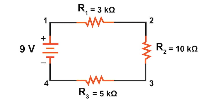
Figure 1. Series circuit with a battery and three resistors.
First, we have to describe the circuit to the computer in a format recognizable by the software. SPICE programs require that all electrically unique points in a circuit be numbered, and component placement is understood by which of those numbered points, or “nodes,” they share.
For clarity, we numbered the four corners of our example circuit of Figure 1 as 1 through 4. SPICE, however, demands that there be a node zero (0) somewhere in the circuit that is typically considered the ground or reference node. So, let’s redraw the circuit, changing the numbering scheme slightly by renumbering the lower-left corner of the circuit from 4 to 0, as shown in Figure 2.
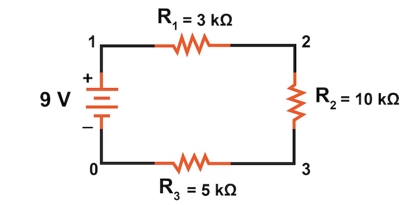
Figure 2. Series circuit with new 0 nodes required for SPICE simulation.
From there, we must enter several lines of text into a computer file describing the circuit in terms SPICE will understand. We will also add a couple of extra lines of code directing the program to perform a DC circuit analysis and to print out voltage and current data for our review. This computer file is known as the netlist in SPICE terminology:
series circuit
v1 1 0
r1 1 2 3k
r2 2 3 10k
r3 3 0 5k
.dc v1 9 9 1
.print dc v(1,2) v(2,3) v(3,0)
.end
Now, all we have to do is run the SPICE program to process the netlist and output the results:
| v1 | v(1,2) | v(2,3) | v(3) | i(v1) |
|---|---|---|---|---|
| 9.000E+00 | 1.500E+00 | 5.000E+00 | 2.500E+00 | -5.000E-04 |
This print output from the SPICE program tells us the battery voltage is 9 V, and the voltage drops across R1, R2, and R3 are 1.5 V, 5.0 V, and 2.5 V, respectively. Voltage drops across any component in SPICE are referenced by the node numbers the component lies between. Thus, v(1,2) references the voltage between nodes 1 and 2 in the circuit, which are the points between R1's location.
Keep in mind that the order of node numbers is important. When SPICE outputs a value for v(1,2), it regards the polarity the same way as if we were holding a voltmeter with the red test lead on node 1 and the black test lead on node 2. We also have a display showing current (albeit with a negative value) at 0.5 mA or 500 μA. This current matches what we previously calculated using Ohm’s Law.
So our mathematical analysis has been vindicated by the computer. This value appears as a negative number in the SPICE analysis due to how SPICE defines current through a voltage source.
SPICE Simulation of a Parallel Circuit
Just as with the series circuit, we can use computer analysis to analyze the parallel circuit shown in Figure 4.
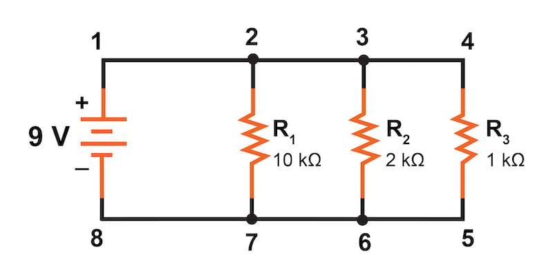
Figure 3. Parallel circuit with a battery and three resistors.
First, we must describe our parallel circuit to the computer in terms it can understand. Let’s start by changing node 8 to 0, as we did for our series circuit analysis above.
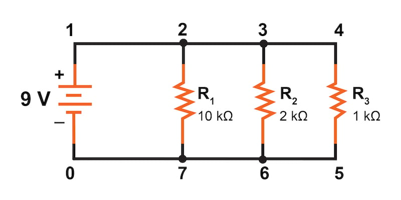
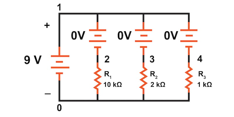
Figure 4. Parallel circuit with new 0 nodes required for SPICE simulation.
In SPICE, all electrically common points must share identical node numbers. In the parallel circuit of Figure 4, we can see that nodes 1, 2, 3, and 4 are electrically common. The same goes for nodes 5, 6, 7, and 0.
With that in mind, let’s consolidate the naming of the bottom electrical node to 0 and the top electrical node to 1. This results in the new circuit diagram of Figure 5.
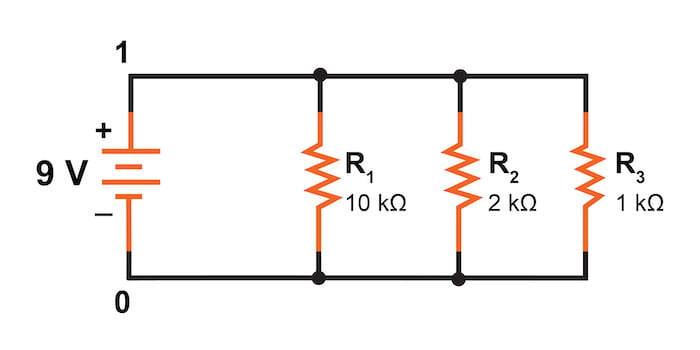
Figure 5. Parallel circuit with consolidated electrically common nodes.
An example like this makes understanding the rationale of node numbers in SPICE fairly clear. By having all components share common sets of numbers, the computer knows they’re all connected in parallel with each other.
To display branch currents in SPICE, we often need to insert zero-voltage sources in series with each resistor and then reference our current measurements to those sources. However, check your SPICE user manual, as many newer versions allow you to display branch currents through other components, including resistors.
For whatever reason, the original creators of the SPICE program made it so that current could only be calculated through a voltage source. This is a somewhat annoying demand of the SPICE simulation program. With each of these “dummy” voltage sources added, some new node numbers (2, 3, 4) must also be created to connect them to their respective branch resistors, as illustrated in Figure 6.

Figure 6. Voltage sources with 0 V and new node numbers were added for the branch's current evaluation.
The dummy voltage sources are all set at 0 V and are ideal sources with 0 Ω resistance, so they have no impact on the circuit operation.
The completed SPICE circuit description file, or netlist, looks like this:
Parallel circuit
 v1 1 0
 r1 2 0 10k
 r2 3 0 2k
 r3 4 0 1k
 vr1 1 2 dc 0
 vr2 1 3 dc 0
 vr3 1 4 dc 0
 .dc v1 9 9 1
 .print dc v(2,0) v(3,0) v(4,0)
 .print dc i(vr1) i(vr2) i(vr3)
 .end
Running the computer analysis, we get the following results, which have been annotated in the printout with descriptive labels:
| v1 | v(2) | v(3) | v(4) |
|---|---|---|---|
| 9.000E+00 | 9.000E+00 | 9.000E+00 | 9.000E+00 |
| Battery | R1 Voltage | R2 Voltage | R3 Voltage |
Voltage
| v1 | i(vr1) | i(vr2) | i(vr3) |
|---|---|---|---|
| 9.000E+00 | 9.000E-04 | 4.500E-03 | 9.000E-03 |
| Battery | R1 Current | R2 Current | R3 Current |
These results from SPICE do indeed match those previously calculated using Ohm’s Law earlier:
$$I_{R1} = 0.9 \text{ mA}$$
$$I_{R2} = 4.5 \text{ mA}$$
$$I_{R3} = 9.0 \text{ mA}$$
Being connected in parallel, these resistors all have the same voltage (9 V) dropped across them.
Series and Parallel Circuit Simulation Using a SPICE Circuit Simulator Review:
- One node in the SPICE circuit must use the number 0; typically, this is the reference or ground node
- All electrically common nodes must use the same circuit node number
- 0 V DC voltage sources can be added in series to evaluate branch currents
Related Content
Learn more about SPICE, series circuits, and parallel circuits in the additional materials down below.
Calculators:
Worksheets:
- Series DC Circuits Practice Worksheet with Answers
- Parallel DC Circuits Practice Worksheet With Answers
- Algebraic Equation Manipulation for Electric Circuits
- Ohm's Law
- Ohm's Law Practice
Video Tutorials and Lectures:
Technical Articles:
- Modeling Hysteresis in SPICE
- Basic Circuit Simulation with LTspice
- How to Simulate Silicon Carbide Transistors with LTspice
- Designing and Simulating EMC Filters with LTspice
- Noise Analysis Using LTspice Tutorial