How Many Hidden Layers and Hidden Nodes Does a Neural Network Need?

So far in this series on neural networks, we've discussed Perceptron NNs, multilayer NNs, and how to develop such NNs using Python. Before we move on to discussing how many hidden layers and nodes you may choose to employ, consider catching up on the series below.

1. How to Perform Classification Using a Neural Network: What Is the Perceptron?
2. How to Use a Simple Perceptron Neural Network Example to Classify Data
3. How to Train a Basic Perceptron Neural Network
4. Understanding Simple Neural Network Training
5. An Introduction to Training Theory for Neural Networks
6. Understanding Learning Rate in Neural Networks
7. Advanced Machine Learning with the Multilayer Perceptron
8. The Sigmoid Activation Function: Activation in Multilayer Perceptron Neural Networks
9. How to Train a Multilayer Perceptron Neural Network
10. Understanding Training Formulas and Backpropagation for Multilayer Perceptrons
11. Neural Network Architecture for a Python Implementation
12. How to Create a Multilayer Perceptron Neural Network in Python
13. Signal Processing Using Neural Networks: Validation in Neural Network Design
14. Training Datasets for Neural Networks: How to Train and Validate a Python Neural Network
15. How Many Hidden Layers and Hidden Nodes Does a Neural Network Need?

 

Hidden-Layer Recap

First, let’s review some important points about hidden nodes in neural networks.

• Perceptrons consisting only of input nodes and output nodes (called single-layer Perceptrons) are not very useful because they cannot approximate the complex input–output relationships that characterize many types of real-life phenomena. More specifically, single-layer Perceptrons are restricted to linearly separable problems; as we saw in Part 7, even something as basic as the Boolean XOR function is not linearly separable.
• Adding a hidden layer between the input and output layers turns the Perceptron into a universal approximator, which essentially means that it is capable of capturing and reproducing extremely complex input–output relationships.
• The presence of a hidden layer makes training a bit more complicated because the input-to-hidden weights have an indirect effect on the final error (this is the term that I use to denote the difference between the network’s output value and the target value supplied by the training data).
• The technique that we use to train a multilayer Perceptron is called backpropagation: we propagate the final error back toward the input side of the network in a way that allows us to effectively modify weights that are not connected directly to the output node. The backpropagation procedure is extensible—i.e., the same procedure allows us to train weights associated with an arbitrary number of hidden layers.

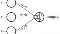
The following diagram summarizes the structure of a basic multilayer Perceptron.

 

 

How Many Hidden Layers?

As you might expect, there is no simple answer to this question. However, the most important thing to understand is that a Perceptron with one hidden layer is an extremely powerful computational system. If you aren’t getting adequate results with one hidden layer, try other improvements first—maybe you need to optimize your learning rate, or increase the number of training epochs, or enhance your training data set. Adding a second hidden layer increases code complexity and processing time.

Another thing to keep in mind is that an overpowered neural network isn’t just a waste of coding effort and processor resources—it may actually do positive harm by making the network more susceptible to overtraining.

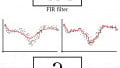
We talked about overtraining back in Part 4, which included the following diagram as a way of visualizing the operation of a neural network whose solution is not sufficiently generalized.  

 

 

A superpowered Perceptron may process training data in a way that is vaguely analogous to how people sometimes “overthink” a situation.

When we focus too much on details and apply excessive intellectual effort to a problem that is in reality quite simple, we miss the “big picture” and end up with a solution that will prove to be suboptimal. Likewise, a Perceptron with excessive computing power and insufficient training data might settle on an overly specific solution instead of finding a generalized solution (as shown in the next figure) that will more effectively classify new input samples.

 

 

So when do we actually need multiple hidden layers? I can’t give you any guidelines from personal experience. The best I can do is pass along the expertise of Dr. Jeff Heaton (see page 158 of the linked text), who states that one hidden layer allows a neural network to approximate any function involving “a continuous mapping from one finite space to another.”

With two hidden layers, the network is able to “represent an arbitrary decision boundary to arbitrary accuracy.”

 

How Many Hidden Nodes?

Finding the optimal dimensionality for a hidden layer will require trial and error. As discussed above, having too many nodes is undesirable, but you must have enough nodes to make the network capable of capturing the complexities of the input–output relationship.

Trial and error is all well and good, but you will need some sort of reasonable starting point. In the same book linked above (on page 159), Dr. Heaton mentions three rules of thumb for choosing the dimensionality of a hidden layer. I’ll build upon these by offering recommendations based on my vague signal-processing intuition.

1. If the network has only one output node and you believe that the required input–output relationship is fairly straightforward, start with a hidden-layer dimensionality that is equal to two-thirds of the input dimensionality.
2. If you have multiple output nodes or you believe that the required input–output relationship is complex, make the hidden-layer dimensionality equal to the input dimensionality plus the output dimensionality (but keep it less than twice the input dimensionality).
3. If you believe that the required input–output relationship is extremely complex, set the hidden dimensionality to one less than twice the input dimensionality.

 

Conclusion

I hope that this article has helped you to understand the process of configuring and refining the hidden-layer configuration of a multilayer Perceptron.

In the next article, we’ll explore the effects of hidden-layer dimensionality using my Python implementation and some example problems.