How to Increase the Accuracy of a Hidden Layer Neural Network

In this article, you'll learn how to modify a hidden layer to improve neural network accuracy using a Python implementation and example problems.

Before we move into that subject, however, consider catching up on the previous entries in this series on neural networks:

1. How to Perform Classification Using a Neural Network: What Is the Perceptron?
2. How to Use a Simple Perceptron Neural Network Example to Classify Data
3. How to Train a Basic Perceptron Neural Network
4. Understanding Simple Neural Network Training
5. An Introduction to Training Theory for Neural Networks
6. Understanding Learning Rate in Neural Networks
7. Advanced Machine Learning with the Multilayer Perceptron
8. The Sigmoid Activation Function: Activation in Multilayer Perceptron Neural Networks
9. How to Train a Multilayer Perceptron Neural Network
10. Understanding Training Formulas and Backpropagation for Multilayer Perceptrons
11. Neural Network Architecture for a Python Implementation
12. How to Create a Multilayer Perceptron Neural Network in Python
13. Signal Processing Using Neural Networks: Validation in Neural Network Design
14. Training Datasets for Neural Networks: How to Train and Validate a Python Neural Network
15. How Many Hidden Layers and Hidden Nodes Does a Neural Network Need?
16. How to Increase the Accuracy of a Hidden Layer Neural Network

 

The number of nodes included in a hidden layer influences the classification ability and speed of a Perceptron neural network. We’re going to run experiments that will help us to formulate some incipient intuition about how hidden-layer dimensionality fits into the attempt to design a network that trains within a reasonable amount of time, produces output values with acceptable latency, and meets accuracy requirements.

 

Benchmarking in Python

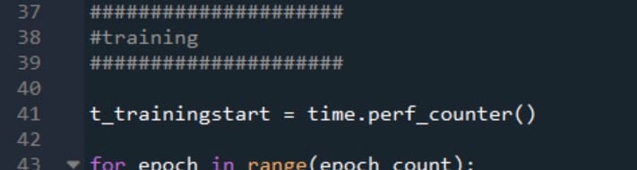
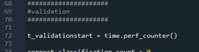
The neural network Python code presented in Part 12 already includes a section that calculates accuracy by using the trained network to classify samples from a validation data set. Thus, all we need to do is add some code that will report execution time for training (which includes feedforward operation and backpropagation) and for the actual classification functionality (which includes only feedforward operation). We’ll use the time.perf_counter() function for this.

This is how I mark the beginning and end of training:

 

 

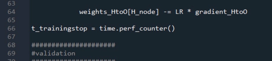
Validation start and stop times are generated in the same way:

 

 

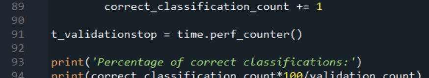
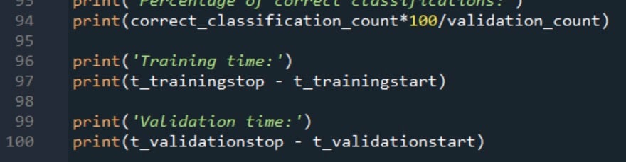
The two processing-time measurements are reported as follows:

 

 

Training Data and Measurement Procedure

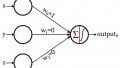
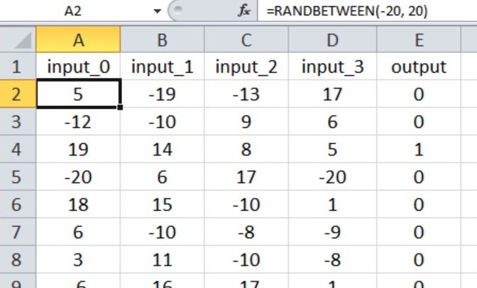
The neural network will perform true/false classification on input samples consisting of four numerical values between –20 and +20.

Thus, we have four input nodes and one output node, and the input values are generated with the Excel equation shown below.

 

 

My training data set consists of 40,000 samples, and the validation set has 5000 samples. The learning rate is 0.1, and I’m performing just one training epoch.

We’ll perform three experiments representing input-output relationships with varying degrees of complexity. The np.random.seed(1) statement is commented out, so initial weight values will vary and therefore so will the classification accuracy.

In each experiment, the program will be executed five times (with the same training and validation data) for each hidden-layer dimensionality, and the final measurements for accuracy and processing time will be the arithmetic mean of the results generated by the five separate runs.

 

Experiment 1: A Low-Complexity Problem

In this experiment, the output is true only if the first three inputs are greater than zero, as shown in the Excel screenshot below (note that the fourth input has no effect on the output value).

 

 

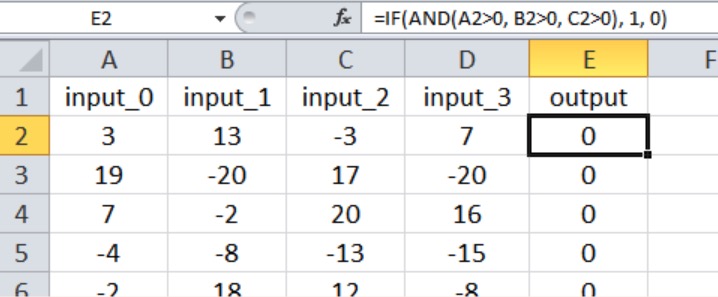
I think that this qualifies as a fairly simple input-output relationship for a multilayer Perceptron.

Based on the recommendations that I provided in Part 15 regarding how many layers and nodes a neural network needs, I would start with a hidden-layer dimensionality equal to two-thirds of the input dimensionality.

Since I can’t have a hidden layer with a fraction of a node, I’ll start at H_dim = 2. The table below presents the results.

 

 

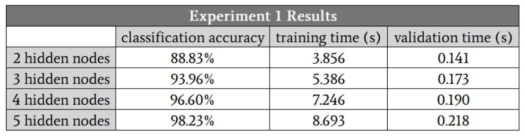
We see classification improvement all the way to five hidden nodes. However, I think that these numbers exaggerate the benefit of increasing from four to five nodes, because the accuracy of one of the four-hidden-node runs was 88.6%, and this dragged down the average.

If I eliminate that low-accuracy run, the average accuracy for four hidden nodes is actually slightly higher than the average for five hidden nodes. I suspect that in this case, four hidden nodes will provide the best balance of accuracy and speed.

Another important thing to notice in these results is the difference in how hidden-layer dimensionality affects training time and processing time. Moving from two to four hidden nodes increases validation time by a factor of 1.3, but it increases training time by a factor of 1.9.

Training is significantly more computationally intensive than feedforward processing, so we need to be particularly mindful of how network configuration influences our ability to train the network in a reasonable amount of time.

 

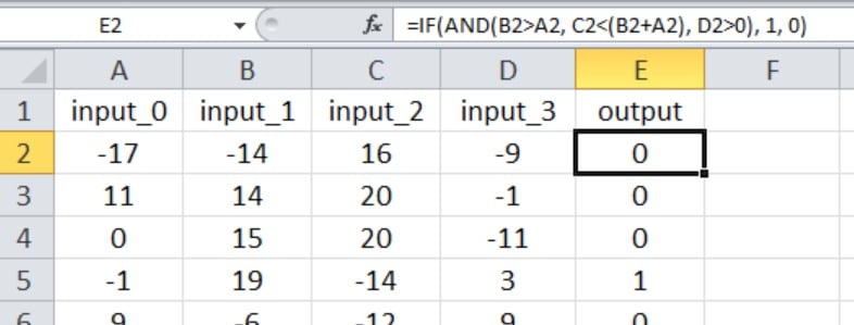
Experiment 2: A Moderate-Complexity Problem

The Excel screenshot shows the input-output relationship for this experiment. All four inputs now influence the output value, and the comparisons are less straightforward than they were in Experiment 1.

 

 

I started with three hidden nodes. Here are the results:

 

 

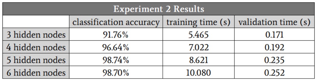
In this case, I suspect that five hidden nodes will give us the best combination of accuracy and speed, though once again the four-hidden-node runs produced one accuracy value that was significantly lower than the others. If you ignore this outlier, the results for four hidden nodes, five hidden nodes, and six hidden nodes look very similar.

The fact that the five-hidden-node and six-hidden-node runs did not generate any outliers leads us to an interesting possible finding: maybe increasing the hidden-layer dimensionality makes the network more robust against conditions that for some reason cause training to be particularly difficult.

 

Experiment 3: A High-Complexity Problem

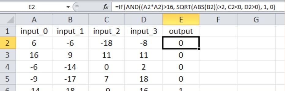
As shown below, the new input-output relationship again includes all four input values, and we have introduced nonlinearity by squaring one of the inputs and taking the square root of another.

 

 

Here are the results:

 

 

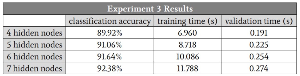
The network definitely had more difficulty with this higher-complexity mathematical relationship; even with seven hidden nodes, the accuracy was lower than what we achieved with only three hidden nodes in the low-complexity problem. I’m confident that we could improve the high-complexity performance by modifying other aspects of the network—e.g., including a bias (see Part 11) or annealing the learning rate (see Part 6).

Nevertheless, I would keep the hidden-layer dimensionality at seven until I was thoroughly convinced that other enhancements could allow the network to maintain adequate performance with a smaller hidden layer.

 

Conclusion

We’ve seen some interesting measurements that paint a fairly clear picture of the relationship between hidden-layer dimensionality and Perceptron performance. There are certainly many more details that we could explore, but I think this gives you some solid foundational information that you can draw upon when you’re experimenting with neural-network design and training.