Understanding ADC Differential Nonlinearity (DNL) Error

The transfer function of a real-world analog-to-digital converter (ADC) might deviate from the ideal response due to effects such as offset and gain errors. Another imperfection that can affect the system response is the ADC’s nonlinearity. Different specifications are commonly used to characterize the linearity of an ADC. For measurement and control applications, differential nonlinearity (DNL) and integral nonlinearity (INL) specifications are helpful performance metrics. When dealing with communications systems, however, the spurious free dynamic range (SFDR) specification is normally a better way to assess the linearity performance of the ADC. 

 

Differential Nonlinearity (DNL)

Diving in, let's look at the blue curve in Figure 1, which shows the ideal transfer function for a 3-bit unipolar ADC.

 

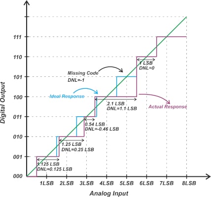
Figure 1. An example showing the ideal transfer function for a 3-bit unipolar ADC. 

 

The ideal response exhibits a uniform staircase input-output characteristic, meaning that each transition occurs at 1 LSB (least significant bit) from the previous transition. In practice, the step width might differ from the ideal value (1 LSB). The purple curve above shows the response of a hypothetical ADC where the steps are not uniform. In this example, the width of code 010 is 1.25 LSB, while the next code exhibits a smaller width of 0.54 LSB. The DNL specification characterizes how the ADC steps deviate from the ideal value.

For an ADC, the DNL of the k-th code is defined by the following equation:

 

\[DNL(k)=\frac{W(k)-W_{ideal}}{W_{ideal}}\]

 

Where W(k) and W_ideal denote the width of the k-th code and the ideal step size, respectively. As an example, for code 1 (or 001) in the above figure, we have:

 

\[DNL(1)=\frac{W(1)-W_{ideal}}{W_{ideal}}=\frac{1.125 \text{ } LSB \text{ } - \text{ }1LSB}{1LSB}=0.125\]

 

This means that the width of code 1 is 0.125 LSB larger than the ideal value. Code 3 (or 011), which has a width of 0.54 LSB, produces a negative DNL of -0.46 LSB. Note that non-ideal code transitions can lead to “missing codes.”

For example, the above ADC doesn’t produce code 5 (101) for any input value. For a missing code, we can assume that the step size is zero, leading to a DNL of -1. Finally, code 6 (110) in our example has the ideal width, i.e. DNL(6) = 0. When calculating the DNL values, we assume that the offset and gain errors of the ADC are already calibrated out. This means that the first and the last transitions occur at the ideal values, and thus, the DNL error is not defined for the first and last steps.

 

Representing ADC DNL Information Using ADS8860

We can represent the above information as a plot of the DNL against the code value. For the above example, we obtain the following plot.

 

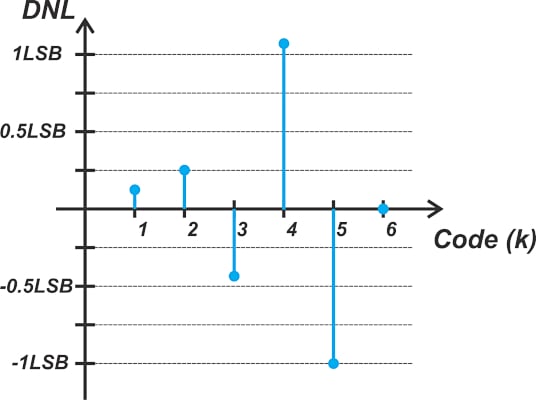
Figure 2. A plot of a DNL against the code value. 

 

DNL is also commonly expressed as minimum and maximum values across all codes. The DNL of our hypothetical ADC is between -1 LSB and +1.1 LSB. Figure 3 shows the typical DNL plot of the ADS8860, a 16-bit successive approximation register (SAR) ADC from TI.

 

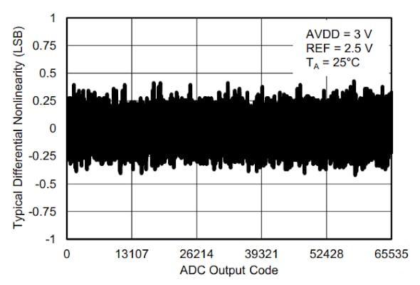
Figure 3. A typical DNL plot of the ADS8860. Image used courtesy of TI

 

The ADS8860 has a maximum DNL of ±1.0 LSB with no missing codes. ADCs that specify a maximum DNL error of +/-1 LSB normally explicitly state whether the device has missing codes or not. “No missing codes” is usually guaranteed. Some ADC datasheets, such as the ADS8860, also provide the DNL vs. temperature plot.

 

Using ADC DNL for Control and Measurement Applications 

To better understand the implications of the DNL specification in control and measurement systems, let’s consider the example depicted in Figure 4.

 

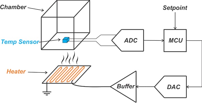
Figure 4. An example feedback system showing the adjustment of the chamber's temperature.

 

In this example, the feedback system attempts to adjust the chamber's temperature. The temperature data is digitized by the ADC and delivered to the processor (MCU). The MCU compares the temperature with the desired value and most likely uses a control scheme such as a PID (proportional-integral-derivative) controller to produce the appropriate input for the digital-to-analog converter (DAC). Finally, the DAC drives the heater through a buffer stage. 

Assume that the chamber temperature is always in the 30 °C to 37 °C range, and we need to measure the temperature with a resolution of 1 °C. Therefore, assuming that the ADC quantization error is the only source of error in our system, we can use a three-bit ADC as it produces the 8 different output codes required by the application. After adjusting the output voltage of the temperature sensor to the input range of the ADC, the 30 °C to 37 °C temperature range will correspond to the 0 to 7 LSB range, as illustrated in Figure 5.

 

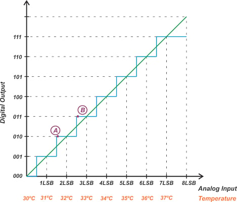
Figure 5. Plot showing the digital output vs analog input and temperature.

 

With an ideal ADC, the steps are uniform, and each transition occurs at 1 LSB from the previous transition (except for the first one). Therefore, the system is guaranteed to detect a 1 °C change in temperature. For example, when the temperature goes from slightly above 31.5 °C (point A in the figure) to slightly above 32.5 °C (point B), the output code changes from 010 to 011. However, assume that the actual ADC doesn’t produce uniform steps and exhibits some DNL error. For example, assume that the ADC has the nonlinear characteristic depicted in Figure 1. How is this going to affect the system's performance? In this case, the system response can be described by the following diagram.

 

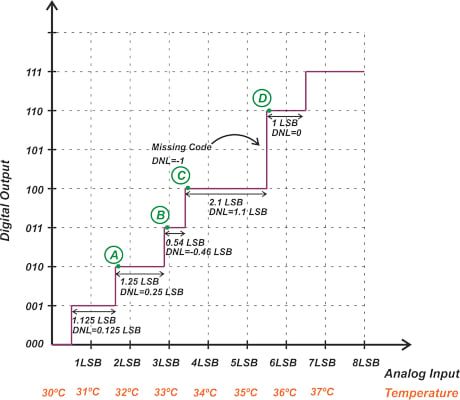
Figure 6. Example system response.

 

Suppose that the temperature is initially at 31.625 °C (point A) and gradually increases. The system is not able to detect a change in temperature until we reach point B at about 32.875 °C. Therefore, the measurement resolution is about 1.25 °C rather than 1 °C. The step corresponding to code 4 is even wider, leading to a local resolution of 2.1 °C.

 

Understanding Converter Resolution vs Accuracy and DNL Error

It’s important to distinguish the resolution problem discussed above from the converter's accuracy. To better understand this, consider the following converter for the chamber example.

 

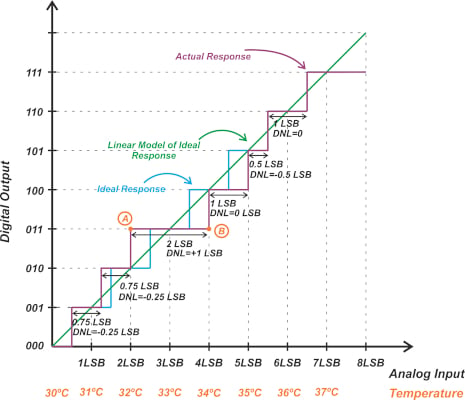
Figure 7. Example showing the chamber's converter responses.

 

Code 3 (011) has a width of 2 LSB, and thus, we know that the local resolution of the system is 2 °C at this point. However, does this mean that the accuracy of the measurement is 2 °C? The above figure shows the ideal staircase response (blue curve) as well as the linear model (green line) of the ideal converter. We can compare the actual response with the linear model to determine the measurement error (or accuracy of the system). 

The maximum deviation of the non-ideal curve from the linear model occurs at points A and B, which is equal to 1 LSB. The error introduced in our measurement is ±1 °C; however, the local resolution is 2 °C. This is because the DNL error can be positive or negative. The net deviation of the actual response from the ideal curve depends on how the positive and negative DNL terms are distributed across the codes. In the above example, two negative DNL errors for codes 1 and 2 are followed by a positive DNL at code 3. This helps the actual response get closer to the ideal curve again. However, in the following example, negative terms accumulate and lead to a larger deviation from the ideal response.

 

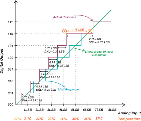
Figure 8. Example responses getting closer to the ideal curve.

 

In this example, the first 5 steps have a DNL of -0.25 LSB, and only code 6 has a positive DNL. As a result, the errors accumulate and lead to a maximum error of 1.75 LSB at point A (from the linear model). While the resolution is close to the previous example (2.25 °C), the measurement error is 1.75 °C (rather than 1 °C in the previous example). 

 

ADC Integral Nonlinearity (INL)

The above discussion shows that the DNL error cannot completely describe the linearity performance of the ADC. The integral nonlinearity (INL) is the specification that characterizes the deviation of the code transition from its ideal value. The INL is defined as the cumulative sum of the DNL error. In mathematical language, the INL of the m-th code is given by:

 

\[INL[m]=\sum_{i=1}^{m-1}DNL[i]\]

 

Just like the DNL, the INL is a vector; however, it is also common to specify only the maximum INL value. For example, the typical and maximum INL of the ADS8860 is ±1.0 LSB and ±2.0 LSB, respectively. 

 

One Final Thought: ADC Noise Impact

It’s worthwhile to mention that code transitions of a practical ADC are affected by the noise present in the system. Figure 9 shows the impact of code transition noise on the ADC characteristic curve.

 

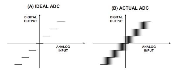
Figure 9. Impact of code transition noise on the ADC characteristic curve, where (A) is the ideal ADC and (B) is the actual ADC. Image used courtesy of Analog Devices

 

As you can see, the transition from one digital code to the next does not occur at exactly one value of the analog input—there’s a small region of uncertainty. In other words, if we measure the transition point from one code to the next several times, we won’t get a single threshold value for the analog input. With today’s moderate to high-resolution ADCs, the code transition noise can be easily comparable with the LSB size. Static specifications such as DNL do not take the noise effect into account.

Therefore, while we understand the importance of the DNL concept in measurement applications, we should note that the code transition noise of a practical ADC can make the DNL specification somewhat less useful in practice. To get around the noise problem, we can use the signal averaging technique. In fact, the test methods for arriving at the DC performance of an ADC inherently use signal averaging, making the measurements less susceptible to the noise effect. 

 

DNL and INL Effect on ADC Dynamic Performance

While we used a control and measurement application to introduce the DNL and INL specifications, these nonlinearity metrics also affect the dynamic performance of the ADC, namely the signal-to-noise ratio (SNR) and the distortion of the ADC. In the next article, we’ll provide some supplementary points about the DNL error and discuss the effect of the DNL and INL errors on ADC’s dynamic response.

 

Featured image used courtesy of Adobe Stock

 

---

 

To see a complete list of my articles, please visit this page.