ADC Nonlinearity—Missing Codes, Monotonicity, and Nonlinearity Effect on SNR

The previous article in this series introduced differential nonlinearity (DNL) and integral nonlinearity (INL) errors in ADCs. In this article, we‘ll discuss eliminating missing codes through averaging, learn about ADC monotonicity, and examine the effect of ADC nonlinearity on the SNR of the system.

 

Eliminating ADC DNL Missing Codes Via Signal Averaging

Signal averaging is a simple but powerful technique that can be used to reduce the noise power in certain measurement applications. Interestingly, averaging can also eliminate “missing codes” of the ADC. This is illustrated in Figure 1.

 

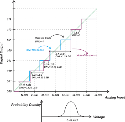
Figure 1. An example plot showing the ADC's missing code.

 

Figure 1 shows the transfer function of a hypothetical nonlinear ADC that misses code 5 (101). With that in mind, we might wonder what output code would be produced if we applied a DC input of 5.5 LSB (least significant bit).

Before answering that, it should be noted that we cannot produce a perfectly noise-free input. At least a small amount of noise will appear at the ADC input, which is actually helpful in our particular situation. Assume that the DC input plus the noise component exhibits the probability density function (PDF) depicted in the lower diagram in the above figure. Note that the mean value of the PDF is equal to the applied DC input (5.5 LSB).

Let’s assume that the noise PDF has a Gaussian distribution with a standard deviation of about \(\frac{LSB}{3}\). This assures that the input is almost always within the input range of codes 100 and 110. With this input, the probability of producing codes 110 and 100 is almost identical. In other words, if we capture the ADC output several times, almost half of the ADC codes will be 110, and the other half will be 100. Therefore, the average of these measurements will be 101. As you can see, averaging can be a system-level solution for eliminating the missing codes of an ADC. In fact, averaging can “smooth” out the DNL errors of the ADC. However, it cannot correct the INL of the ADC.

One might ask: could averaging remove the missing code if the standard deviation of the Gaussian distribution was larger than \(\frac{LSB}{3}\)? Also, what if the noise component was not Gaussian at all and had an arbitrary PDF?

In these more general cases, the output code produced by averaging depends on the DNL of the adjacent codes of the missing code as well as the actual noise PDF. However, in a real-world design, we should be able to remove missing codes through averaging.

 

Signal Averaging: a Special Type of Dithering

In the above example, the inherent noise of the system enables the averaging process to improve the resolution of the system. To better understand this, consider a perfectly noise-free DC input. In this case, the system would produce the same code no matter how many times we repeated our measurement. If the output is the same, averaging will do nothing for us. This might seem counter-intuitive that some level of noise can actually be helpful in certain situations. While the above example relied on the inherent noise of the system, it is also possible to deliberately add some noise to the ADC input to improve its linearity or resolution. This technique is known as dithering. The common averaging technique can be considered a special type of dithering.

 

Transfer Function Monotonicity

Previously (in the article linked in the introduction), we discussed how the DNL error can change the local resolution of the ADC when dealing with measurement and control applications such as the one depicted below in Figure 2.

 

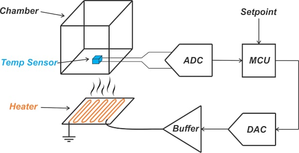
Figure 2. Example measurement and control application. 

 

Non-monotonicity of the transfer function is another type of non-ideality that can be problematic in closed-loop systems. The following example (Figure 3) depicts a non-monotonic three-bit ADC.

 

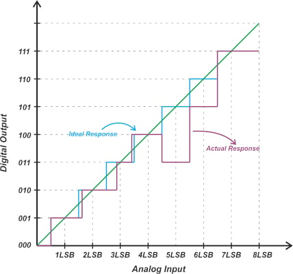
Figure 3. An example plot of a non-monotonic three-bit ADC.

 

The output of a monotonic ADC is non-decreasing for an increase in the input value. This is not the case in Figure 3. In this example, the output code decreases from 100 to 011 as we increase the input from 4 LSB to 5 LSB. In a closed-loop system, non-monotonicity can change negative feedback to positive feedback and cause instability and oscillation. As a result, designers of such systems need to make sure that the ADC is monotonic. Keep in mind that DNL is not defined at non-monotonic steps.

  

ADC DNL Less than -1 LSB

Thus far, we have had examples where the ADC DNL is as small as -1 LSB (for example, when the ADC has a missing code). You might wonder if it is possible to have a DNL less than (or more negative) than -1 LSB? The following diagram from a Maxim Integrated tutorial illustrates an example (Figure 4) where the ADC has a DNL of -1.5 LSB.

 

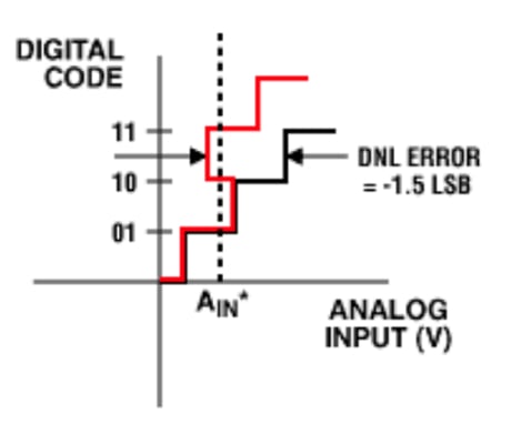
Figure 4.  Example diagram showing an ADC with a DNL of -1.5 LSB. Image used courtesy of Maxim Integrated/ADI 

 

According to this tutorial, the output code produced at A_IN* can be one of three possible values; and when the input voltage is swept, code 10 will be missing.

It seems that this is a rare type of error. ADC course notes from trusted experts, such as Haideh Khorramabadi and Boris Murmann, mention that DNL less than -1 is not possible and consider it to be undefined. Also, note that the common DNL definition discussed in the previous article doesn’t yield a DNL of -1.5 LSB for the above example. The equation for calculating the DNL of the k-th code is repeated below for convenience:

 

\[DNL(k)=\frac{W(k)-W_{ideal}}{W_{ideal}}\]

 

Here, W(k) and W_ideal denote the width of the k-th code and the ideal step size, respectively. We normally consider the step width (W(k)) to be positive, leading to a minimum DNL of -1 LSB. For the above example, we can get a DNL of -1.5 LSB only if we assume that the step width is -0.5 LSB.

While a DNL less than -1 LSB is considered to be undefined, the maximum of the ADC DNL can exceed +1 LSB and has no upper boundary. Also, it’s worth mentioning that, unlike ADCs, D/A converters (DACs) can have a DNL of less than -1 LSB. This is shown below in Figure 5.

 

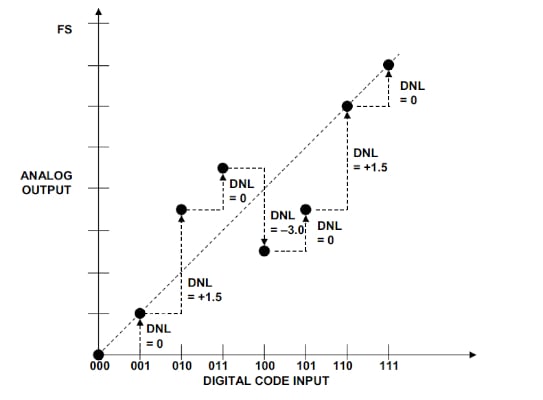
Figure 5. An example plot showing a DAC that has a DNL of less than -1 LSB. Image used courtesy of Analog Devices

 

How DNL and INL Affect ADC Signal-to-noise Ratio

We have thus far examined the effect of DNL and INL, mainly on control and measurement applications. The nonlinearity of the ADC transfer function also manifests itself as an increase in the noise level of the system.

Since an ADC represents a continuous range of analog values through several discrete levels, this inherently adds an error known as the quantization error. By subtracting the analog equivalent of the output code from the input voltage, we can find the quantization error. Figure 6 shows a ramp input (with a slope of one) that increases from zero volts to the full-scale value of a three-bit ADC.

 

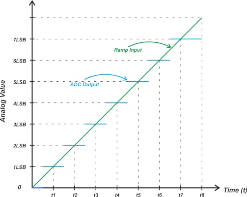
Figure 6. Example plot showing a ramp input that increases from zero volts to the full-scale value.

 

Figure 6 also shows the analog equivalent of the ADC output codes. If we subtract these two curves, we obtain the following quantization error, shown in Figure 7.

 

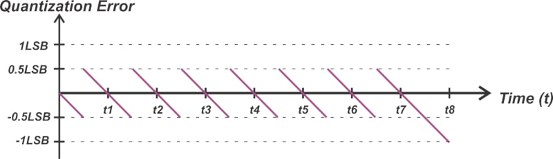
Figure 7. Example showing the quantization error vs time. 

 

Except for the last step, the quantization error of an ideal ADC is always between ±0.5 LSB. For most practical applications, the quantization error of an ideal ADC can be modeled as a noise source with a uniform amplitude distribution in the ±0.5 LSB range. The average power of the quantization noise is $$\frac{LSB^2}{12}$$. However, what if the steps are not uniform?

For example, consider applying the ramp input to the nonlinear transfer curve depicted in Figure 1. This is illustrated in Figure 8.

 

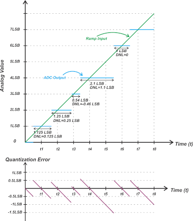
Figure 8. Example plot showing the application of the ramp input to the nonlinear transfer curve.

 

The lower curve in Figure 8 provides the plot of the quantization error for this non-ideal case. Since the steps are not uniform, the limits of the quantization error are not the same for different codes. In this particular example, the quantization error can be as negative as about -1.5 LSB.

For a nonlinear ADC, the transition points of the quantization error are offset from the ideal transition values by the INL error of the code. The above example suggests that DNL/INL can change the quantization noise of the ADC.

 

Nonlinearity-induced Noise Term

There are different methods for deriving the nonlinearity-induced noise term. However, the end result is that the ADC nonlinearity can be modeled as an additive noise term at the ADC input. If we assume that the DNL error has a uniform distribution over the ±DNL range, the PDF of the DNL error will be as shown in Figure 9.

 

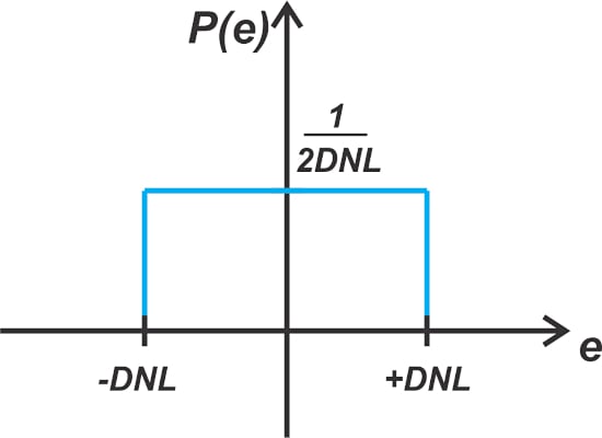
Figure 9. Example showing the PDF of the DNL error with a uniform distribution over the ±DNL range.

 

Since the integral of the probability density function is equal to one, its value will be $$\frac{1}{2DNL}$$ for – DNL < e < + DNL, as shown in the equation below:

 

\[P_{DNL \text{ } Noise}=\int_{-DNL}^{+DNL}e^{2}P(e)de=\int_{-DNL}^{+DNL}e^{2}\frac{1}{2DNL}de=\frac{DNL^{2}}{3}\]

 

Assuming that the DNL error and the quantization error are independent, the total noise power from these two effects is given by:

 

\[P_{Noise} = P_{Quantization}+P_{DNL \text{ } Noise}=\frac{LSB^2}{12}+\frac{DNL^{2}}{3}\]

 

Now we can calculate the SNR. With a full-swing sine-wave input, the amplitude of the input signal is half the full-scale value $$(\frac{2^N LSB}{2})$$, which yields a signal power of:

 

\[P_{Signal}=\frac{1}{2}{\big(\frac{2^{N}LSB}{2}\big)}^{2}\]

 

Where N is the number of bits of the ADC. Therefore, the signal-to-noise due to quantization and DNL error can be found by the following equation:

 

\[SNR=\frac{\frac{1}{2}{\big(\frac{2^{N}LSB}{2}\big)}^{2}}{\frac{LSB^2}{12}+\frac{DNL^{2}}{3}}\]

 

You can find a somewhat different method of obtaining this equation in Haideh Khorramabadi’s course notes. As an example, if DNL = 0.5 LSB, the above equation yields:

 

\[SNR=\frac{\frac{1}{2}{\big(\frac{2^{N}}{2}\big)}^{2}}{\frac{1}{12}+\frac{0.5^{2}}{3}}\]

 

Expressed in dB, we obtain Equation 1:

 

\[SNR=6.02N-1.25\]

Equation 1.

 

The SNR of an ideal ADC (with uniform steps) is given by the following well-known equation in Equation 2:

 

\[SNR=6.02N+1.76\]

Equation 2.

 

Comparing Equations 1 and 2, we observe that a DNL of ±0.5 LSB reduces the SNR by 3.01 dB. Note that the above derivation is based on the assumption that the DNL error has a uniform distribution. This might not be the case in practice; however, this analysis allows us to estimate the SNR performance in presence of nonlinearity. Also, the assumption of independence of the "DNL-noise" and quantization noise is less valid at higher values of the DNL error. Equation 3, below, shows another derivation for calculating the average power of the nonlinearity-induced noise in ADCs:

 

\[P_{Noise} = P_{Quantization}+P_{Nonlinearity \text{ } Noise}=\frac{LSB^2}{12}+\frac{LSB^{2}}{2^N}\sum_{i=0}^{2^N-1}\Big(INL(i)\Big)^2\]

Equation 3.

 

A relatively straightforward analysis similar to that of the uniform quantization noise can be used to derive the above expression. For more information, you can also refer to the papers “Statistical Analysis of ENOB and Yield in Binary Weighted ADCs and DACs With Random Element Mismatch” by J. A. Fredenburg and “Noise Sensitivity of the ADC Histogram Test” by P. Carbone.

 

Featured image used courtesy of Adobe Stock

 

---

 

To see a complete list of my articles, please visit this page.