Facebook
 Google
 GitHub
 Linkedin
Transient Analysis in SPICE
In transient analysis, we convert the input voltage Vin to a pulse, sinusoidal, or piecewise linear source instead of a DC or AC voltage. We then look at the output over a period of time rather than over a voltage or frequency range.
To learn about transient analysis, we will use the same circuit as we did in our previous AC and DC analysis: the bipolar buffer repeated here in Figure 3-6.
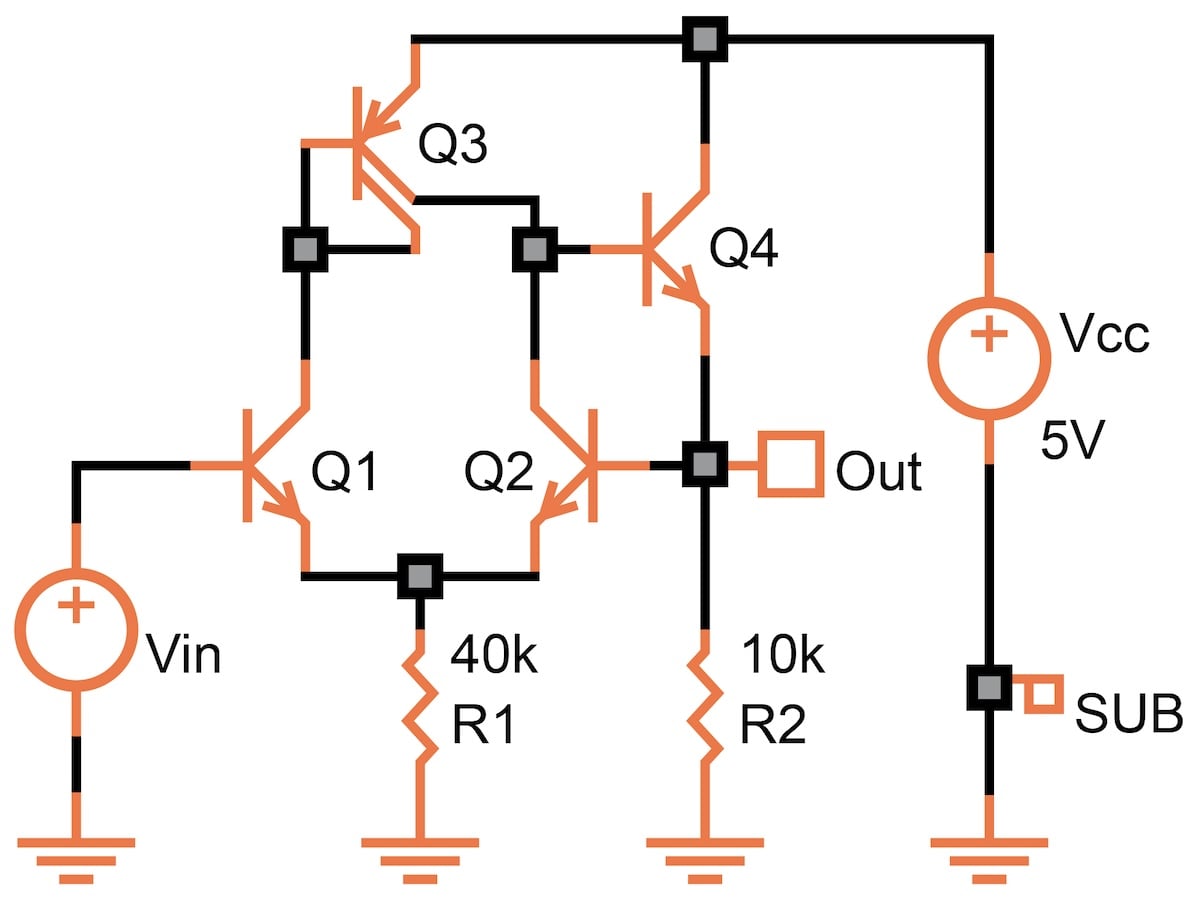
Figure 3-6. A simple example of a bipolar buffer for transient simulation. [click to enlarge]
Figure 3-7 shows the result of a transient analysis with a 1 V pulse at the input.
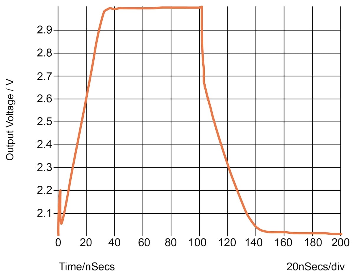
Figure 3-7. Transient analysis: output voltage from a 1 V pulse at the input. [click to enlarge]
You may have to make a few trial runs to get the appropriate pulse width and total analysis time. At first, the program will choose its own timesteps, shortening the intervals when a lot of changes happen and lengthening them when no changes are taking place. But if you’re not satisfied with the resolution, you can dictate what maximum (or minimum) timestep it is allowed to take.
Figure 3-8 shows a transient analysis where the 1 V input has been changed to a sine wave at 1 kHz.
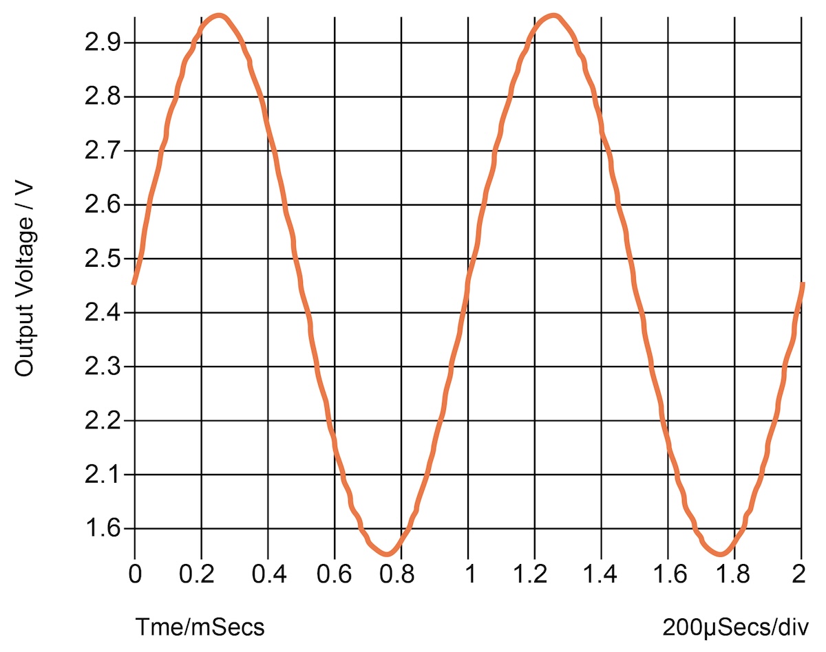
Figure 3-8. Transient analysis 2: output voltage from a 1 Vpp sine-wave at the input. [click to enlarge]
Changing the input to a sine wave will help you learn a great deal more about the circuit. It will be immediately obvious if the circuit can reproduce the waveform without clipping it at either the high or low excursions. That’s only a rough impression of fidelity, however. What you need to know is the amount of distortion in the waveform.
In some programs, you simply display the sine wave, click on the distortion button, and get the result. But if you want to have all the information, nothing beats a Fourier Analysis.
Fourier Analysis
The Fast Fourier Transform (FFT) is a routine that extracts the frequency components from a waveform. It’s rather tricky to use and sometimes produces errors.
Figure 3-9 shows the result of a continuous Fourier analysis, which is both more detailed and more reliable than the FFT.
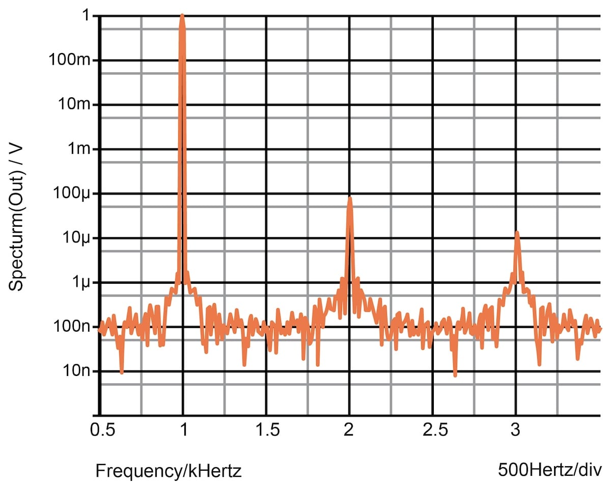
Figure 3-9. Continuous Fourier analysis frequency spectrum. [click to enlarge]
What we see in the graph is amplitude versus frequency. At 1 kHz is the fundamental frequency, which has an amplitude of nearly (but not quite) 1 V. At 2 kHz is the second harmonic, with an amplitude of 100 µV, or 0.01%. The third harmonic measures about 12 µV, or 0.0012%.
To get this kind of resolution, you need to run the sine wave for many cycles (at least 1,000) with small enough timesteps.
Transient Noise Analysis
Noise analysis in the small-signal (AC) mode has strict limitations. It presumes that the operating voltages and currents are steady. This is fine for a circuit that is perfectly linear, but it falls down if a design is nonlinear, either by design or by mishap.
Take, for example, the case of a mixer (or modulator). A signal of a particular frequency enters a deliberately nonlinear block: for example, a diode mixer or the phase detector of a phase-locked loop. The nonlinearity creates other frequencies—usually much lower ones, such as the frequency difference between the two input signals. We typically use and amplify one of those new frequencies.
An AC noise analysis is useless here because it can’t follow what happens to the noise as it’s transformed by the mixer. What we need is a transient analysis program that pays attention to noise sources. Few have this capability—a notable exception, again, is Simetrix.