Facebook
 Google
 GitHub
 Linkedin
Simulating Device and Process Variation in SPICE
Device parameters in an IC vary from run to run and from wafer to wafer. The devices are made at temperatures at which the material is no longer a semiconductor. You have to wait for the wafer to cool down to measure the parameters of a diffusion.
Most parameters follow a "normal," or Gaussian, distribution. This distribution is illustrated in Figure 3-10.
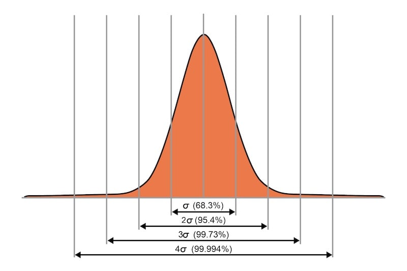
Figure 3-10. The normal, or Gaussian, distribution.
In a normal distribution, the number of occurrences is maximum at the mean value. A deviation of ±σ (sigma) from this point contains 68.3% of all measured values. If you allow the deviation to be three times as large (±3σ), you enclose 99.73% of all measurements.
This sounds like you’re discarding only 0.27% of all values, but the figure is deceiving—we’ve considered only one parameter, when there are many in an integrated circuit. Suppose your design is influenced by 50 parameters: the total parameter "yield" is then .997350, or 87.4%. This means you would discard 12.6% of all chips on a wafer.
Unless you simply don't care about cost, you need to design an analog IC so no chips are lost because of parameter variations. In other words, the design needs to withstand a variation of each and every device parameter to at least 3σ. Even then, 4σ would be better.
But how do you find out how much parameter variation your design can take?
Four-Corners Analysis
Some designers use what’s called a "four-corner analysis." In a four-corner analysis, device parameters are bundled together in four groups, which represent extremes or worst cases. The plain fact is this: it doesn't work for analog circuits.
The four-corner models are just barely able to predict the fastest or slowest speed of digital ICs, but the groupings simply don't apply to analog ones. In fact, no grouping is possible–a parameter's influence differs from design to design. Analog designers who are satisfied with a four-corner analysis simply fool themselves into believing that they have a handle on variations when, in truth, the result is quite meaningless.
Monte Carlo Analysis
The answer is Monte Carlo analysis and only Monte Carlo analysis. A true Monte Carlo analysis varies the device parameters in a random fashion so that every combination of variations is covered. This is also what you get in production.
You don't need to vary every parameter of a device, only the major ones. For example, varying the saturation current (IS), beta factor (βF), and the capacitances in a bipolar transistor model is sufficient. The same is true for the threshold voltage (VTH), the transconductance (gm), and the capacitances in MOS transistors.
If matching is expected, there must be two additional entries:
- One for the absolute variation.
- One for the variation between devices on the same chip.
These "tolerances" are either inserted into the model file directly or contained in a separate file, depending on the analysis program used. The Monte Carlo program then simply runs the chosen analysis repeatedly, each time with a different set of variations, randomly chosen. For example, Figure 3-11 shows the variation over temperature for an untrimmed bandgap reference.
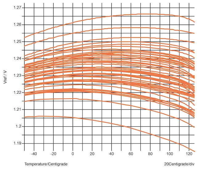
Figure 3-11. Monte Carlo analysis of an untrimmed bandgap reference over temperature.
How many runs need to be specified for a Monte Carlo analysis? There’s an easy way to find out: start with 20, then increase this number until the extremes no longer change. For this analysis, 50 runs were used, which is more than we needed. With today's fast computers, you can afford to go overboard, though—the analysis took all of 8 seconds!
This one picture gives you the variation of a reference voltage over temperature exactly as it will happen in production. Notice that there’s a Gaussian distribution (more curves at the center, fewer at the extremes). Between the top and bottom curves lie 99.73% (3σ) of all circuits.
Without the Monte Carlo analysis, we wouldn’t know how much variation to expect until several wafers from several different lots have been tested. A single prototype wafer can’t tell you what the variations in production will be.