Facebook
 Google
 GitHub
 Linkedin
AC Analysis in SPICE
The one thing you never want to forget about a SPICE AC analysis is this: the signal is treated as if it were insignificantly small. You may specify a 1 V input signal—most people do this because it represents 0 dB and is thus very convenient—but the analysis program will process it without disturbing any of the bias levels.
If you have a high gain—60 dB, say—the output plot will show a voltage of 1,000 V without even blushing. The AC analysis is intended to show you the gain relative to the input. The actual values, taken out of context, are often absurd.
To examine AC analysis, we'll use the bipolar buffer in Figure 3-3. This is the same circuit we used in the DC analysis.
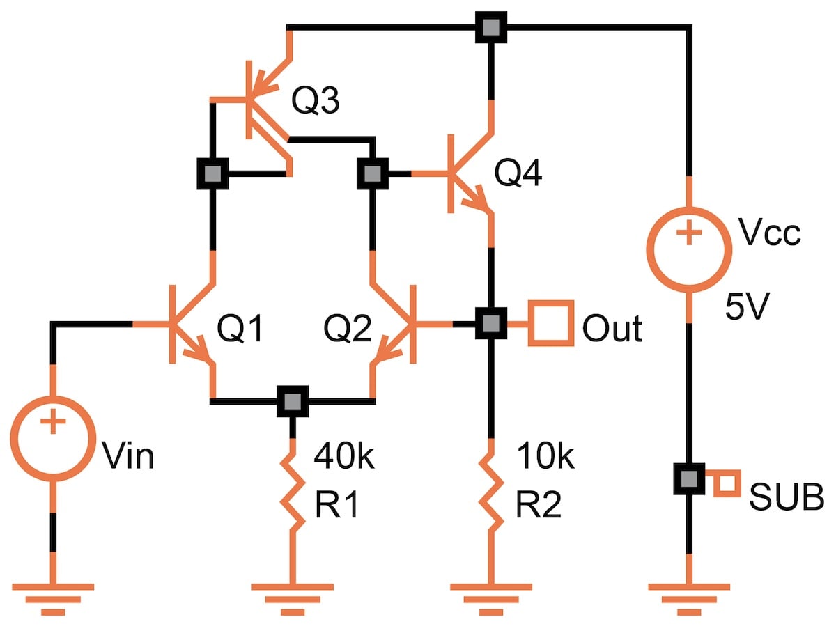
Figure 3-3. A simple example of a bipolar buffer for AC simulation. [click to enlarge]
Figure 3-4 shows the output response of our buffer using the most simple AC analysis: a 1 V AC signal at the input on top of a DC voltage of 2 V, with the frequency swept from 200 kHz to 200 MHz. The output is in dB relative to the input, so 0 dB is a "gain" of 1, and –3 dB is a "gain" of 0.708 (or a loss of 29.2%).
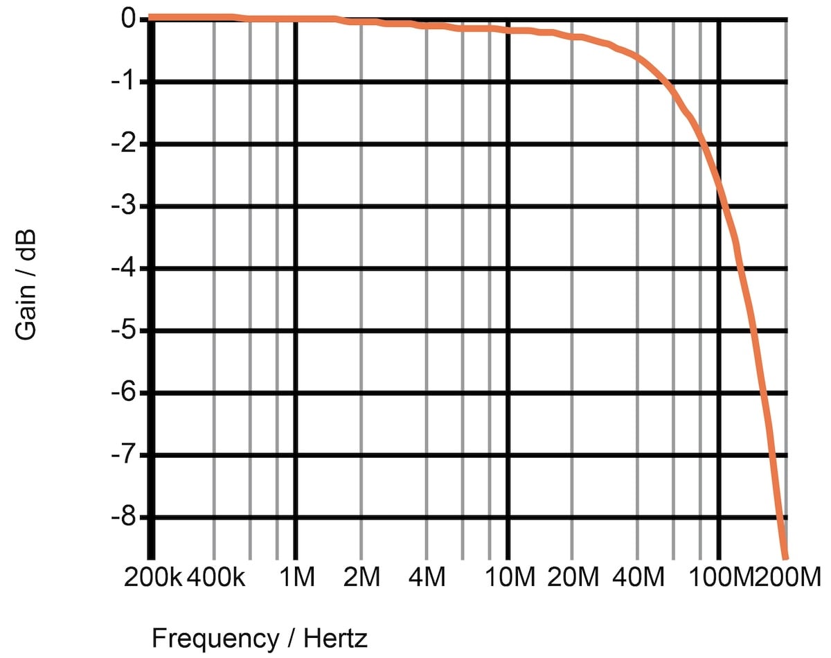
Figure 3-4. AC analysis: gain (in dB) vs. frequency. [click to enlarge]
We could also move the AC source into the Vcc supply to measure how much of a supply's ripple gets into the output. However, make sure there's only one AC source per circuit during your simulations.
With equal ease, you can measure the AC response of an output current relative to an input current. But when it comes to the relationship between a voltage and a current, a measurement in dB makes little sense.
SPICE also lets you measure the phase of any voltage or current relative to the phase of an input signal. This is of particular interest in circuits which employ feedback. We’ll discuss this more in the Analog Measurements and Op Amps chapters.
Remember, though, that this is a small-signal analysis, done at one particular bias point. The actual AC response—particularly the phase—may be different since a real-life signal changes the operating voltages and currents.
Noise Analysis
SPICE also supports the simulation of circuit noise. It is similar to AC analysis. Here, the AC source is turned off, and the combined effect of all noise sources inside the circuit (resistors, currents) at the output is displayed. Figure 3-4 shows an example of the output noise vs. the frequency.
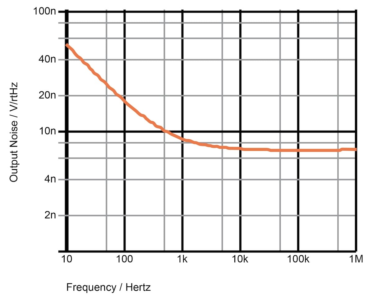
Figure 3-5. Output noise vs. frequency. [click to enlarge]
The measure is nV/√Hz or μV/√Hz. Despite the awkward name, it’s, in fact, an elegant measure. To get the actual noise (usually in μVrms), you simply multiply the value taken from the curve by the square root of the frequency interval of interest.
For example, between 100 Hz and 1 kHz, we read an average of about 12 nV/√Hz. Multiply this by the square root of 900, and you get 360 nVrms of noise. This is the noise value if you use a bandpass filter that cuts out everything below 100 Hz and above 1 kHz.
Similarly, we would measure about 24 nVrms in the flat (white noise) region between 10 kHz and 1 MHz. Even though the curve has a lower value, the total noise is much larger because of the wider frequency range.