Facebook
 Google
 GitHub
 Linkedin
Basic Amplifier Configuration (Part 1)
Video Lectures created by Tim Feiegenbaum at North Seattle Community College.
We're in Section 11.2 and we're looking at basic amplifier configurations.
There are two basic op amp configurations in wide use, they are the inverting amplifier and the non-inverting amplifier.
These configurations form the basis for many other related applications.
First, we're going to look at the non-inverting amplifier circuit.
Non-Inverting Amplifier Circuit
Typically, power supply terminals are omitted from schematic diagrams with op amps. Typically, you do not see the power supplies here. There is a component here, I think I'll mention it, this is RB and RB is a biasing component. Something you might notice here, we have a signal that is being applied to this input. Remember that we have infinite impedance here and this particular component is only there as a balancing component for this one.
Remember that we had that current, though it was very small, that actually came out of the bases of the differential amp and it flowed out of the inputs. Remember that that current flowing across R1 will create a tiny voltage. This component RB is only placed there to offset whatever voltage is developed on R1 due to those currents. But for purposes of calculation, this value can actually be ignored.
Back to our circuit identification.
If the signal is applied to the inverting input, that is going to be the minus side, then the output will be inverted.
If the signal is applied to the non-inverting input, then the output will not be inverted.
Op Amp Analysis Rules
First, the open-loop gain of an op amp is extremely high. Remember we talked about 100,000 to 1,000,000, sometimes larger.
Second, the output voltage of an op amp responds to the difference in potential between its two inputs. Remember the op amp amplifies the difference.
Third, the output voltage swing is limited to within 1-3 V of the supply voltage and we looked at that in a previous discussion.
We have a couple of rules.
The difference in voltage between the input pins of an op amp is zero as long as the amplifier output is not driven to one of its extremes. Basically, what that means is in linear operation, as long as we don't go into saturation at either end, the voltage difference will be 0 volts. Second rule: The input pins of an op amp are open circuits and draw no current from the external circuit. If we apply a voltage to the op amp, the impedance is so large that no current will flow into the op amp. Again, this is because the impedance of the op amp is ideally infinite.
Circuit Operation
Here we have a non-inverting amplifier. As the input pins on an op amp are essentially open circuits, there is no voltage drop across RB. We've talked about RB already. Since input impedance is infinite, the voltage drop across the biasing resistor is effectively 0 volts. Unless specifically addressed, the value of RB can be ignored.
RF and R1 form a voltage divider across the output voltage. Here we have this voltage divider across the output. Since feedback is formed, a result of voltage divider action gain is this: RF divided by R1 plus 1 will give us our output. Here we have this voltage divider, a portion of that is fed back to the input. We're going to look at … I'm just going to jump ahead just for a moment. This is actually that circuit in use in Electronics Workbench. Let's analyze this before we go look at the actual circuit. If we said that RF was 10K and that R1 was 2K and that we had a 100 millivolt input, what is our output going to be? We have this formula, RF over R1 plus 1. We're going to say that would be 10K divided by 2K plus 1. The 10K over 2K is going to be 5 plus 1, that says that the gain of this amplifier will be 6. If we have a gain of 6, we have a 100 millivolt input, that means that our V out should be 600 millivolts.
There is a way that we can confirm that through some of the rules that we previously talked about. We said that the difference in voltage here is effectively zero. We also mentioned that concept of a virtual short. Whatever value is felt here will also be felt right here. If we apply that, we could say that 100 millivolts will be felt across this component, which is 2K. That will generate a current and since no current flows into the op amp, all of that current will flow through both of these components. If we calculate that current and then take that current times 12K, we should get this value. Let's quickly pull up our calculator and see if, in fact, that happens.
We'll say 100 exponents minus 3, that will give us 100 millivolts and we will divide that by 2000 ohms, 2K, and that gives us the current that is going to be felt through R1. Now we have that current, that current is going to flow through both components. If we take that value times 12 exponent 3 and there we have it, 600 millivolts. That is our circuit analysis for this particular amplifier going to the non-inverting input.
This is the actual circuit. In fact, you have this in your package of circuits with Multisim and I took this directly from your package and, again, the thing is it is drawn in such a way that it's not readily recognizable. Notice here the non-inverting input is on the top and here it is on the bottom. The 2K and the 10K are now connected to the negative. Here we've got the power supply, the negative is connected over here to pin four, positive is connected down here to pin seven. Pins one and five are unused and then pin six comes out here. Then we have the o-scope connected to actually look at the outputs and pin … The blue line here is going to the output of pin six and the red is going over here to the input.
What you might note, this is a screen capture of the oscilloscope readout and we're on a scale of 200 millivolts per division. Since this is coming in at 100 millivolts, we would expect that to be exactly half of one square and that's what it is. You'll notice that this value has nothing to do with it. This actually is the RB value, which can be ignored. You'll notice that it has no impact because we have 100 millivolts in and that's what you see, there's nothing dropped there, and that's what we would expect. On the output, at 200 millivolts per square, we have one, two, three squares and that would give us our 600 millivolt output with an input of 100 millivolts.
Effects of Negative Feedback
This is negative feedback. We amplify a signal and then we feed back a portion of it and that is negative feedback. So what are we going to say? The portions of the output signal return to the input cause a cancellation of the effects of the input voltage. Negative feedback controls the voltage gain of an op amp. It establishes it, in the case of that previous amp, A equaled 6. Closed-loop voltage gain is more stable than open-loop voltage gain and provides a wider bandwidth. What I've done, this came, actually, from the first section in this particular chapter but, here, again, we see this graph of gain versus bandwidth and in this particular circuit, A was 6 and if we converted that to 20 log of 6, we'd get about 15.5 decibels and that is actually this value right here, the closed-loop voltage gain.
What we'll see here is that we don't have a mighty gain but we do have great bandwidth and our bandwidth goes from zero hertz all the way out to 1000 kilohertz. We lose our gain but we gain wide bandwidth. We have a very stable gain all the way across this spectrum. From zero hertz all the way to 100K Hertz, we have a gain of 6 or 15.5 dB.
This concludes our introduction to the non-inverting amp. Let's see, what did we look at? We looked at the graph of gain versus frequency and we looked at actual simulation and then we looked at the schematic for that simulation and we looked at some of the rules regarding op amp analysis and then we formally looked at the non-inverting amplifier. In the next section, we will look at the inverting amplifier.