Introduction to the Memory Effect in RF Power Amplifiers

Two previous articles in this series discussed analog and digital predistortion for power amplifiers (PAs). As we learned, predistortion compensates the PA’s nonlinearity by placing a nonlinear circuit before its input. The digital form of this technique is considered one of the most effective methods of RF power amplifier linearization.

To design high-performance predistorters, we need to include the memory effect in our models. In this article, we’ll delve into the effect of memory within RF power amplifiers. We’ll examine its various manifestations and the techniques for its measurement and observation, as well as briefly touching on the fundamental reasons for this phenomenon.

 

What is the Memory Effect?

For predistortion to work, we need an accurate characterization of the PA’s nonlinear behavior. If the PA’s output is solely a function of its present input, this is relatively simple. In practice, however, the output of a PA is a function of both present and past input values. This phenomenon, known as the memory effect, is illustrated in Figure 1.

 

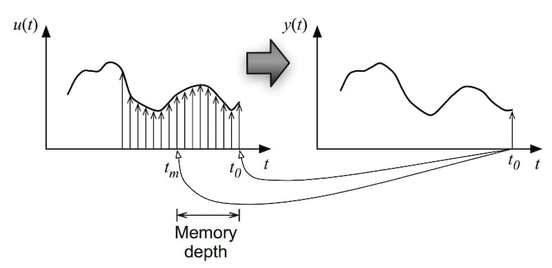
Figure 1. Due to the memory effect, the output is a function of both present and past input values. Image used courtesy of John Wood

 

When the memory effect comes into play, the nonlinear response of the PA is no longer static. Instead, it changes with time. In Figure 2, for example, the memory effect takes the form of hysteresis in the PA response.

 

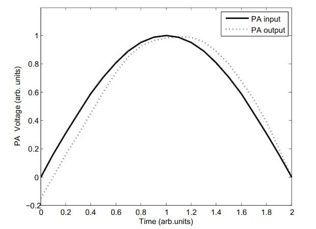
Figure 2. Hysteresis effect in the response of an RF power amplifier. Image used courtesy of John Wood

 

Here, a given input value yields different outputs depending on whether the signal is rising or falling.

The presence of the memory effect in PAs might initially surprise electrical engineers. However, it’s important to recognize the range of circuits—from basic RC circuits to digital FIR filters—that display dependency on historical input values. For example, consider the RC circuit shown in Figure 3.

 

Figure 3. The transient response of a simple RC circuit can’t be determined without knowing the past input values. Image used courtesy of Steve Arar

 

The transient output voltage of the above circuit at a given time can’t be solely described by the input voltage excitation at that time. We need to know the input signal’s past values as well. Capacitors and inductors introduce memory into analog circuits.

 

Four Fundamental Categories of Electrical Circuits

For a clearer comprehension of the matter, it should be noted that electrical systems can be broadly classified into four key categories:

1. Linear without memory.
2. Linear with memory.
3. Nonlinear without memory.
4. Nonlinear with memory.

For example, a circuit composed solely of linear resistors is a linear, memoryless system. A network comprising linear resistors along with a linear energy storage component, such as a capacitor or inductor, results in a linear system with memory.

A combination of linear and nonlinear resistors constitutes a nonlinear, memoryless system. However, pairing a nonlinear resistor with a linear energy storage device—a linear capacitor, for instance—creates a nonlinear system with memory. A single energy storage element with nonlinear properties, like a nonlinear capacitor, also falls into the category of nonlinear systems with memory.

In the frequency domain, the memory effect makes the gain and phase shift of both linear and nonlinear systems frequency-dependent. In the time domain, the memory effect causes the system's response to be dependent upon previous input values.

 

What Causes the Memory Effect in PAs?

There are several different mechanisms that can produce a memory effect in PAs, starting with the wide dynamic variation in transistors’ parasitic capacitances and inductances. The frequency dependence of the bias and matching circuits can also cause memory effects. Other mechanisms include thermal effects, semiconductor trapping effects, and modulation of the supply rails.

 

Measuring the Memory Effect

PAs processing wideband signals with non-constant amplitudes exhibit both static distortions and memory effects. The static nonlinearity is relatively easy to measure: we only need to connect the PA’s output to a spectrum analyzer with sufficient dynamic range and resolution bandwidth.

To observe the memory effect, we commonly use the more complex test setup in Figure 4.

 

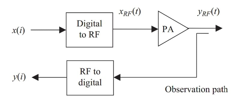
Figure 4. The PA’s output is demodulated and digitized for a direct comparison with the original input signal. Image used courtesy of Richard N. Braithwaite

 

In the above diagram, x(i) and y(i) denote the digital input and output signals. The observation path used to produce y(i) consists of a coupler to sample the PA’s output and a receiver to convert the RF signal to its corresponding digitized value.

Once we know the values of x(i) and y(i), we can apply techniques such as mean squared error (MSE) to estimate the PA’s nominal gain. Deviations from the nominal gain are caused by the PA’s nonlinearity. Figure 5 shows we can study the PA’s saturation behavior by plotting the output magnitude as a function of the input magnitude.

 

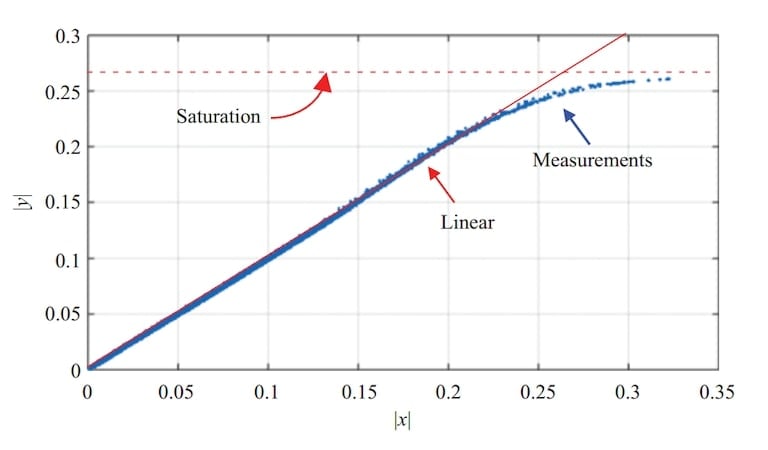
Figure 5. The typical transfer characteristic of a nonlinear PA with memory effect. Image used courtesy of Richard N. Braithwaite

 

At higher input levels, the output begins to saturate, meaning that the output no longer increases linearly with the input. This reduction in gain at elevated power levels is referred to as gain compression.

Having x(i) and y(i), we can also measure AM-to-AM (amplitude-modulation-to-amplitude modulation) and AM-to-PM (amplitude-modulation-to-phase-modulation) responses of the PA. As we’ll discuss in the next section, we can use these characteristics to quantify the dispersion of practical PAs. A power amplifier with dispersion will have more than one output value for a given input value. Unlike gain compression, which is a form of static nonlinearity, dispersion is caused by the PA’s memory effect.

 

AM-to-AM and AM-to-PM Responses in the Presence of the Memory Effect

The gain of the PA at an input value of x(i) is given by:

$$G \big (x(i) \big )~=~\frac{y(i)}{x(i)}$$

 

The AM-to-AM response is defined as the magnitude of the PA’s gain versus the magnitude of the input. Similarly, the AM-to-PM response is the phase of the PA’s gain versus the input magnitude.

In order to evaluate the PA’s performance, we first create the required baseband signal and transfer it to an arbitrary waveform generator (AWG). The AWG modulates and upconverts the baseband signal to the radio frequency. We then apply this RF signal to the PA and capture its output with a vector signal analyzer, which converts the signal back to the baseband and digitizes it.

By comparing the original and processed baseband signals, we can effectively analyze the memory effect of the PA. As an example, Figure 6 shows some measurement results from the paper “A Novel Weighted Memory Polynomial for Behavioral Modeling and Digital Predistortion of Nonlinear Wireless Transmitters” by A. E. Abdelrahman.

 

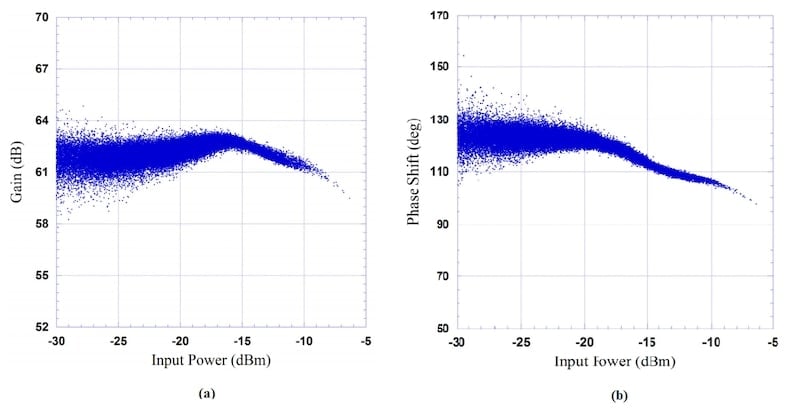
Figure 6. The measured AM/AM (a) and AM/PM (b) characteristics of a PA with memory effect. Image used courtesy of A. E. Abdelrahman

 

To obtain these measurements, the researchers applied a long-term evolution (LTE) test signal to the PA. They then determined the instantaneous complex gain of the PA by comparing the input and output signals. This enabled them to generate the AM/AM and AM/PM characteristics using the modulated test signal.

As this example demonstrates, real-world PAs may show considerable dispersion in gain magnitude and phase. The dispersion plotted above is more pronounced at lower input power levels. In order to ensure that the observed output dispersion isn’t caused by the input signal power distribution, we also need to check the input’s probability density function (PDF). The PDF of the input test signal for the above experiment is shown in Figure 7.

 

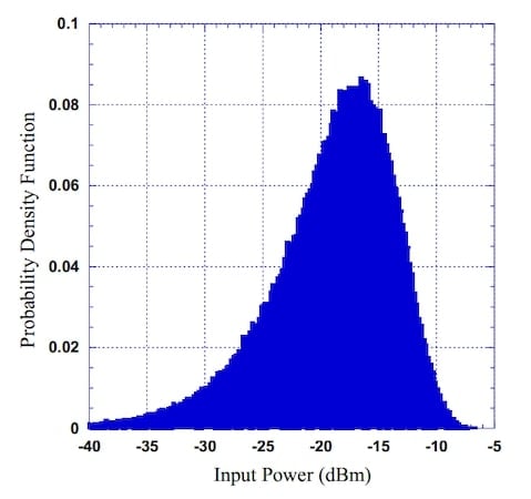
Figure 7. Probability density function of the LTE test signal. Image used courtesy of A. E. Abdelrahman

 

The test signal's PDF shows lower values at reduced power levels, such as –30 dBm, compared to –15 dBm. However, the AM/AM and AM/PM characteristics display greater dispersion at an input level of –30 dBm than at –15 dBm. This confirms that the dispersion stems from the PA's memory effect, not the input power distribution.

 

Challenges for Predistortion Linearization

A predistortion circuit needs to exhibit the inverse transfer characteristic of the PA. The combined response of the predistorter/PA then becomes linear. If the PA’s behavior is quasi-static, identifying the appropriate predistortion function is more straightforward. In this case, we can assume that the PA’s output amplitude has a fixed, monotonic relationship to the input signal.

In the absence of the memory effect, the output signal's value is solely determined by the present input value. Consequently, it's possible to record the PA's nonlinear behavior and encode this data into a look-up table, which can then be utilized to implement a digital predistortion system like the one in Figure 8.

 

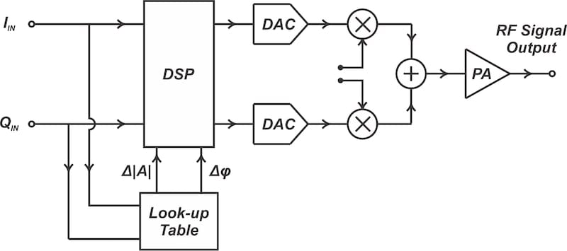
Figure 8. An open-loop, LUT-based predistortion system. Image used courtesy of Steve Arar

 

If the memory effect is present, however, we need to model the PA's memory effects. Techniques for doing so include the Volterra series, Wiener models, and memory polynomial models. We then incorporate these models in our predistortion linearizer.

 

Wrapping Up

The memory effect causes dispersion in the PA's transfer characteristics, affecting both the AM/AM and AM/PM responses. The AM/AM characteristic indicates the magnitude of the instantaneous gain; the AM/PM characteristic specifies the gain's phase. We can use modulated test signals to measure the PA’s memory effect under realistic conditions.

Because the memory effect complicates the task of characterizing the PA, it degrades the performance of predistortion linearization methods. To correct for the short-term memory effect, more advanced digital predistortion algorithms may include some of the recent history of the signal.

 

This article is Part 4 in a series on linearization techniques and nonlinearity in RF systems. Below is a complete list of articles in this series:

1. Introduction to the Feed-Forward Linearization of RF Power Amplifiers
2. Using Analog Predistortion for RF Power Amplifier Linearization
3. Improving RF Power Amplifier Linearity With Digital Predistortion
4. Introduction to the Memory Effect in RF Power Amplifiers
5. Using the 1 dB Compression Point to Characterize RF System Nonlinearity
6. Understanding Intermodulation Distortion and the Third-Order Intercept Point in RF Systems
7. A Guide to Calculating IM3 and IP3 for Nonlinear RF Circuits
8. Understanding Dynamic Range and Spurious-Free Dynamic Range in RF Systems
9. Understanding the Third-Order Intercept Point of a Cascaded System
10. Dynamic Nonlinearity in RF Power Amplifiers: Insights From Two-Tone Testing

 

​​​​​​​Featured image used courtesy of Adobe Stock