DC Lab - An Analog Computer For Averaging

Project Overview

Digital computers, such as personal computers (PCs), calculators, and smartphones, perform mathematical operations in a series of discrete steps. Analog computers perform calculations in a continuous fashion, exploiting Ohm’s and Kirchhoff’s Laws for arithmetic purposes. The answer in an analog computer is computed as fast as voltage propagates through the circuit—ideally, at the speed of light!

In this surprisingly simple project, you will build and test the analog computer, illustrated in Figure 1, to compute the average of three input voltages. 

 

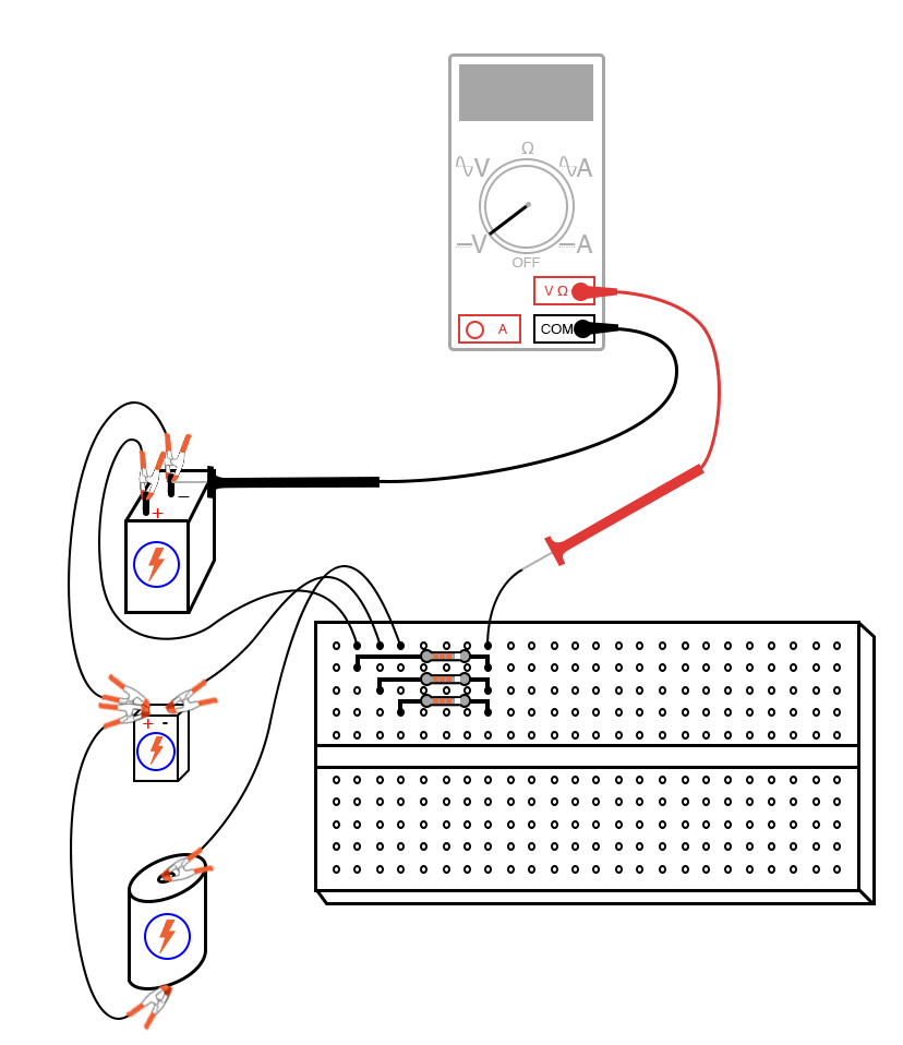
Figure 1. Analog computer for averaging calculation built on a breadboard.

 

Parts and Materials

• Three batteries, each one with a different voltage
• Three equal-value resistors, between 10 kΩ and 47 kΩ each. When selecting the resistors, measure each one with an ohmmeter and choose three that are the closest in value to each other. Precision is very important for this experiment!

 

Learning Objectives

• Learn how a resistor network can function as a voltage signal averager
• Introduction to analog computing
• Illustrate the application of Millman’s Theorem

 

Instructions

Step 1: Build the analog computer averaging circuit, as shown in the schematic diagram of Figure 2. 

 

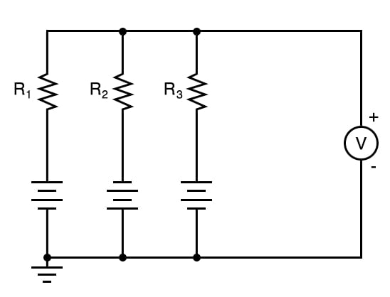
Figure 2. Circuit schematic of an analog computer averaging circuit

 

You can construct it using a breadboard, as illustrated in Figure 1, or using terminal strips, as illustrated below in Figure 3. 

 

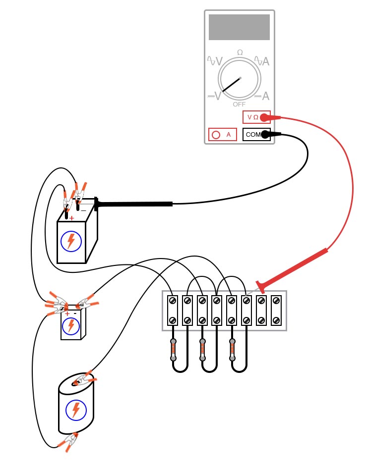
Figure 3. Analog computer for averaging calculation built on using terminal strips

 

Pay careful attention to notice that the battery connected to resistor R₂ is connected backward to the other two with the negative side up.

Step 2: Measure all battery voltages with a voltmeter and record the values. When you measure each battery voltage, keep the black test probe connected to the ground point (the side of the battery directly joined to the other batteries by jumper wires), and touch the red probe to the other battery terminal. Polarity is important here! The voltage of the second battery connected to resistor R₂ should read as a negative quantity when measured by a properly connected digital meter, the other batteries measuring positive.

Step 3. Calculate the average of the three battery voltages: \( (V_1 + V_2 + V_3) / 3 \).

Step 4: Connect the voltmeter at the point shown in the schematic and illustrations and measure the voltage. It should register the algebraic average of the three batteries’ voltages. If the resistor values are chosen to match each other very closely, the output voltage of this circuit should match the calculated average closely as well. This deceptively crude circuit performs the function of mathematically averaging three voltage signals together and so fulfills a specialized computational role. In other words, it is a computer that can only do one mathematical operation: averaging three quantities together.

Step 5: Disconnect one battery and remeasure the output voltage. It will equal the average voltage of the two remaining batteries.

Step 6: Connect the jumper wires formerly connecting the removed battery to each other to effectively create a 0 V input for that branch of the circuit, as illustrated in Figure 4. 

 

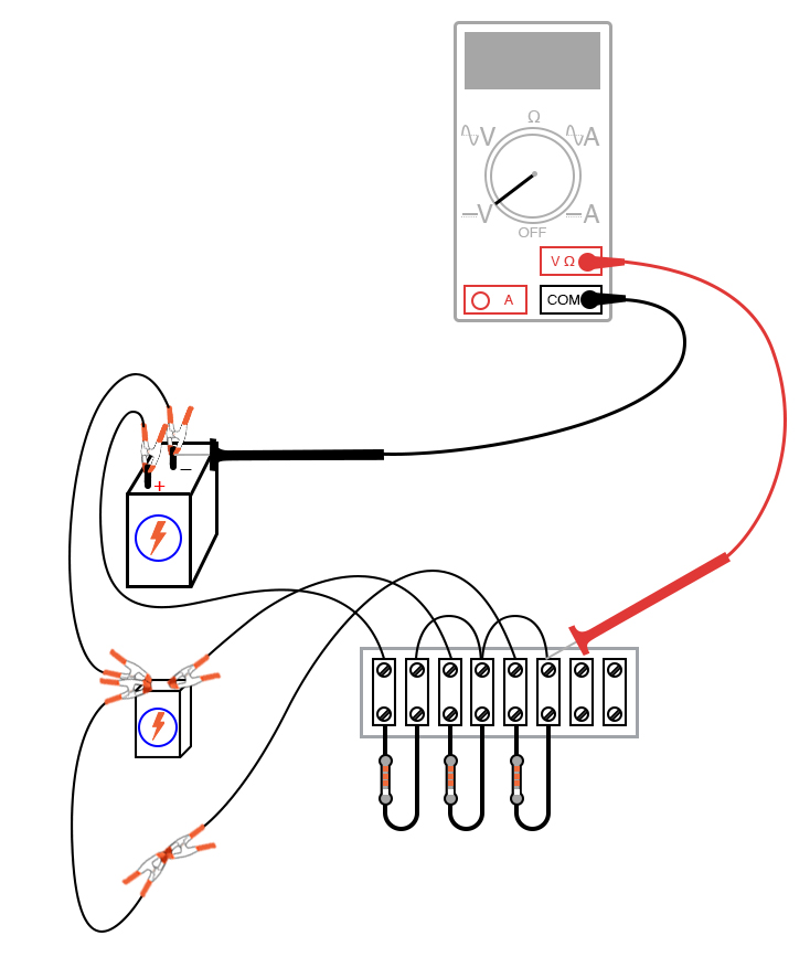
Figure 4. Applying 0 V to one branch of the analog computer averaging circuit

 

The circuit will average the two remaining battery voltages together with 0 V, producing a smaller output signal.

The sheer simplicity of this circuit deters most people from calling it a computer, but it undeniably performs the mathematical function of averaging. Not only does it perform this function, but it performs it much faster than any modern digital computer can! At one time, analog computers were the ultimate tool for engineering research; however, since then, they have been largely supplanted by digital computer technology. Digital computers enjoy the advantage of performing mathematical operations with much better precision than analog computers, albeit at much slower theoretical speeds.

With the addition of circuits called amplifiers, voltage signals in analog computer networks may be boosted and re-used in other networks to perform various mathematical functions. Such analog computers excel at performing the calculus operations of numerical differentiation and integration and, as such, may be used to simulate the behavior of complex mechanical, electrical, and even chemical systems.

 

SPICE Simulation of an Analog Computer Circuit

We can also simulate our analog computer circuit in SPICE. We can force a digital computer to simulate an analog computer, which averages three numbers together. Obviously, we aren’t doing this for the practical task of averaging numbers, but rather to learn more about circuits and more about computer simulation of circuits!

 

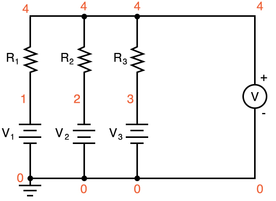
Figure 5. Adding node numbers to the analog computer circuit for SPICE simulation.

 

Netlist (make a text file containing the following text, verbatim):

 

Voltage averager
v1 1 0 
v2 0 2 dc 9 
v3 3 0 dc 1.5 
r1 1 4 10k 
r2 2 4 10k 
r3 3 4 10k 
.dc v1 6 6 1 
.print dc v(4,0) 
.end 

 

Related Content

Learn more about the fundamentals behind this project in the resources below.

 

Calculators:

• Ohm's Law Calculator

 

Textbook:

• Analog Computational Circuits
• DC Network Analysis
• Millman's Theorem

 

Worksheets:

• Millman’s Theorem Worksheet
• Voltmeter Use Worksheet
• Kirchhoff's Laws Worksheet