Vol. DIY Electronics Projects

Chapter 3 DC Circuit Projects

DC Lab - Rate-of-change Indicator

In this hands-on electronics experiment, you will build an analog differentiator circuit that outputs a signal proportional to the rate-of-change and learn about one of the advantages of analog circuits.

Project Overview

The circuit in Figure 1 will provide a demonstration of using analog circuits to perform mathematical computations.

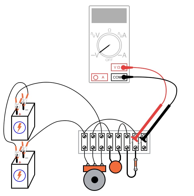
Analog rate-of-change differentiator circuit

Figure 1. Analog rate-of-change differentiator circuit.

We typically only think of digital circuits, like our computers, as methods for mathematical computation. However, as you will see, analog circuits can also be used to perform some complex mathematical operations using surprisingly simple circuitry.

Parts and Materials

Two 6 V batteries or 12 V power supply
Capacitor, 0.1 µF
1 MΩ resistor
Potentiometer, single turn, 5 kΩ, linear taper

The potentiometer value is not especially critical, although lower-resistance units will, in theory, work better for this experiment than high-resistance units. I’ve used a 10 kΩ potentiometer for this circuit with excellent results.

Learning Objectives

Learn how to build a differentiator circuit
To obtain an empirical understanding of the derivative calculus function

Instructions

Step 1: Build the circuit illustrated in Figure 1 and represented in schematic form in Figure 2.

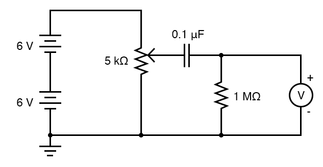
Schematic diagram for the differentiator circuit

Figure 2. The schematic diagram for the differentiator circuit is illustrated in Figure 1.

Step 2: Measure the voltage between the potentiometer’s wiper terminal and the ground point shown in the schematic diagram (the negative terminal of the lower 6 V battery). This is the input voltage for the circuit.

Step 3: Adjust the potentiometer and see how it smoothly varies between zero and 12 V as the potentiometer control is turned to full range. Since the potentiometer is used here as a voltage divider, this behavior should be unsurprising to you.

Step 4: Measure the voltage across the 1 MΩ resistor. What does the voltmeter indicate while the potentiometer is not being moved?

Step 5: For this and the following steps, a digital voltmeter is highly recommended, and I advise setting it to a very sensitive (millivolt) range to obtain the strongest indications. Turn the potentiometer slowly clockwise and note the voltmeter’s reading.

Step 6: Turn the potentiometer slowly counter-clockwise and note the voltmeter’s indication. What difference in magnitude and sign do you see between the two different directions of potentiometer control motion?

Step 7: Try turning the potentiometer at faster rates in both directions. How does the voltmeter's output change?

Step 8: Try moving the potentiometer so that the voltmeter gives a steady, small indication. What kind of potentiometer motion provides the steadiest voltage across the 1 MΩ resistor?

In calculus, a function representing the rate of change of one variable as compared to another is called the derivative. This simple circuit illustrates the concept of the derivative by producing an output voltage proportional to the input voltage’s rate of change over time. Since this circuit performs the calculus function of differentiation with respect to time (outputting the time derivative of an incoming signal), it is called a differentiator circuit. The capacitor placed in series blocks DC (constant) voltages while passing AC (changing) voltages.

Like the averaging circuit project, the differentiator circuit is a kind of analog computer. Differentiation is a far more complex mathematical function than averaging, especially when implemented in a digital computer. Thus this circuit is an excellent demonstration of the elegance of analog circuitry in performing mathematical computations.

More accurate differentiator circuits may be built by combining resistor-capacitor networks with electronic amplifier circuits. To learn more about computational circuitry, go to the analog integrated circuits chapter.