Facebook
 Google
 GitHub
 Linkedin
Applying the t-Test to Engineered Systems
This article provides an example of how we can use t-testing to determine if an experiment has produced a statistically significant change in system performance.
This article is Part 13 in a collection of articles on statistics in electrical engineering. We've covered a lot so far, so if you're just now joining the series, please be sure to review the list of topics below.
- Analyzing statistics as an electrical engineer
- Descriptive statistics
- Descriptive statistical measures: average deviation, standard deviation, and variance
- Introducing the normal distribution
- The Gaussian distribution, histograms, and probability
- The Gaussian cumulative distribution function in statistical analysis
- Parametric tests, skewness, and kurtosis
- Three ways to find statistical relationships
- Introducing the t-distribution to find statistical significance
- Understanding statistical significance in data analysis
- Using correlation coefficients to find statistical relationships
- Understanding t-values and testing for statistical significance
A Lab Hypothetical: What's Causing High PER?
Let’s imagine that we’re developing a wireless communication system. The system consists of a transmitter that sends packetized digital data to a receiver, and our primary means of quantifying performance is the packet error rate (PER). The receiver uses a cyclic redundancy check (CRC) to identify and discard packets that have one or more erroneous bits, and the PER is simply the ratio of discarded packets to received packets.
We’ve been testing and characterizing the system in the lab for months, and consequently, we have an abundance of room-temperature performance data.
We know that when the system is operating in the lab and is configured with attenuation corresponding to the maximum specified range, it achieves an average PER of 0.001, i.e., for every 1,000 received packets, one packet must be discarded.
Statistical Troubleshooting
Unfortunately, we’ve conducted multiple field tests during the last few weeks, and the system didn’t perform very well.
There was no obvious cause for the higher PER, and no patterns were immediately apparent. Thus, we’ll need to create some troubleshooting experiments in an attempt to track down the problem(s). Various things change when a system moves from the lab to the field, but since the field tests took place in Death Valley, temperature is a likely culprit.
Our plan is to crank up the thermostat in the lab and gather some PER data. The system is not intended to operate at extreme temperatures, so we don’t need to test at 125°C or even 70°C. We’ll try 40°C, and since it’s expensive to keep the lab at this temperature for long periods of time, we won’t be able to gather large quantities of data.
...three days later…
We’ve gathered nine 40°C PER measurements. Each measurement represents the PER observed during a two-hour period of operation. In other words, we heated up the lab, activated the system, let it run for two hours, and recorded the PER.
Then we deactivated the system, allowed it to remain inactive for a while, reactivated it, and recorded a new PER datum for a new two-hour period of operation. With three two-hour testing periods per day for three days, we have nine data points.
Here are the PER values that we obtained:
| PER |
|---|
| 0.0010290 |
| 0.0010113 |
| 0.0010380 |
| 0.0010198 |
| 0.0009702 |
| 0.0010486 |
| 0.0010503 |
| 0.0009941 |
| 0.0010067 |
By just looking at the measurements, we can see that the PER tends to be higher than the room-temperature value of 0.001, but we need to examine the data more carefully to determine if the change in PER is statistically significant.
Performing the t-Test
A t-test requires a t-value, and we saw in the previous article that we calculate a t-value as follows:
\[t=\frac{\bar{x}-\mu}{s/\sqrt{n}}\]
where \(\bar{x}\) is the sample mean, μ is the population mean (or more generally, some reference value serving as a point of comparison), s is the sample standard deviation, and n is the sample size.
In this experiment μ = 0.001, i.e., the room-temperature PER. The sample size is 9, and with some help from Excel, I can quickly find the sample mean and the sample standard deviation: \(\bar{x} = 0.001018667 \) and s = 2.62881×10⁻⁵. Thus,
\[t=\frac{0.001018667-0.001}{2.62881\times10^{-5}/\sqrt{9}}\approx 2.13\]
Now we have our t-value. The next step is to find the threshold against which this t-value will be compared; we call this the critical value, denoted by t*. The three pieces of information that we need are the degrees of freedom (denoted by ν) of our experimental data, the significance level, and whether we will perform a one-tailed or two-tailed test.
I think that 5% (⍺ = 0.05) is a reasonable significance level for an experiment like this one, and ν = n – 1 = 8. We’re assuming that increasing the temperature either will have no effect or will degrade the PER; it won’t improve the PER. Thus, we will perform a one-tailed test.
Looking at our table of t-distribution critical values, we see that t* = 1.86.
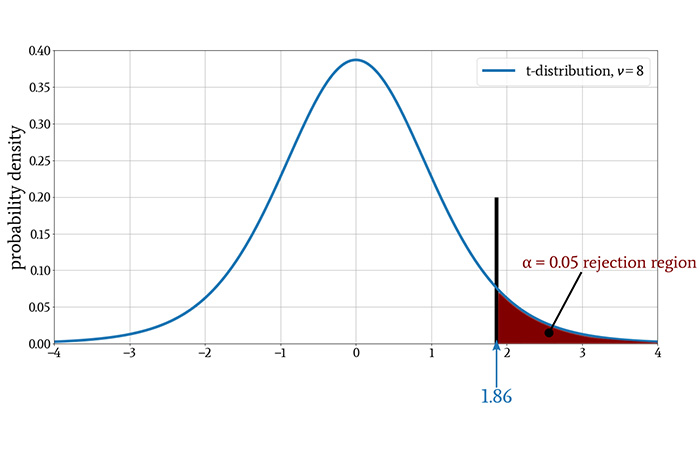
The null hypothesis in our experiment states that there is no meaningful relationship between temperature and PER. Our obtained t-value of 2.13 is greater than 1.86 and is, therefore, in the rejection region of the distribution. Thus, we reject the null hypothesis and claim that there is indeed a relationship between the variables of interest: higher temperature is correlated with higher PER.
Conclusion
We’ve worked through a straightforward example of significance testing as a technique for troubleshooting an electronic system. We’ll extend this imaginary experiment into the next article as we continue our exploration of the t-test.
Related Content