Understanding t-Values and Testing for Statistical Significance

Welcome to All About Circuits' series on the role of statistics in electrical engineering. If you're new to the series, you'll find a list of topics we've covered so far below. Otherwise, please read on to learn how t-values can help us determine whether a relationship exists between variables in experimental data. 

1. Introduction to statistical analysis in electrical engineering
2. Introduction to descriptive statistics in electrical engineering
3. Three descriptive statistical measures in signal processing
4. Using Bessel’s correction in standard deviation calculations
5. The normal distribution
6. The normal distribution, histograms, and the probability mass function
7. Obtaining the Gaussian cumulative distribution function for statistical analysis
8. Tests in the normal distribution: skewness, kurtosis, and parametric tests
9. Correlation, causation, and covariance
10. Finding statistical relationships using the Pearson and Spearman correlation coefficients
11. What is statistical significance?
12. Understanding the t-distribution in tests for statistical significance

The Purpose of the t-Distribution

If you’ve read the previous article, you know that we can use the t-distribution instead of the normal distribution to model the null hypothesis for the purpose of assessing statistical significance. The t-distribution is advantageous when we’re working with a small sample size because in such cases it produces a more accurate confidence interval.

The shape of the t-distribution changes according to the parameter \(\nu\), which denotes degrees of freedom and is determined by the sample size (denoted by n):

\[\nu=n-1\]

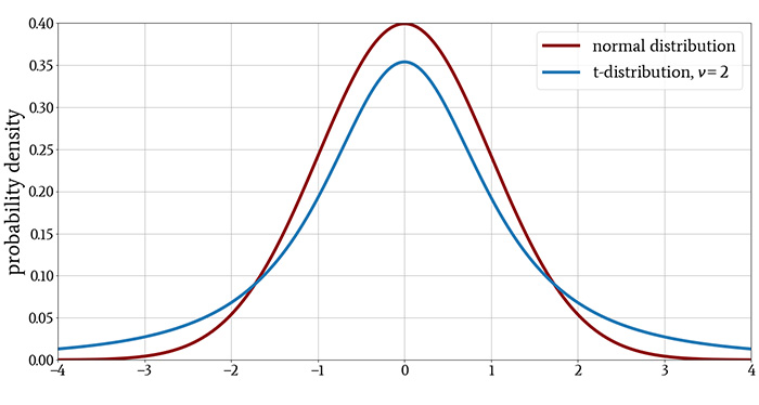
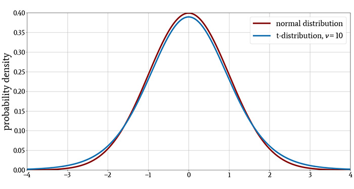
For a small sample size, the t-distribution has heavier tails than the normal distribution, indicating a higher probability of observing values that are far from the mean. For larger sample sizes, the difference between the t-distribution and the normal distribution is increasingly negligible.

These characteristics are evident in the following plots.

What Is a t-Test?

When we perform a t-test, we use the t-distribution to model the null hypothesis. A t-test is a method of assessing statistical significance by comparing the means of dependent-variable distributions observed during an experiment.  

A t-test requires that the independent variable be bivariate, i.e., having only two possible values. For example, if the independent variable in an experiment is temperature, we can use a t-test if we need to analyze data associated with only two temperatures. If we collected data at three or more temperatures, we would need to use a different statistical test called a one-way analysis of variance (ANOVA).

As you may recall from a previous article, statistical tests come in both parametric and nonparametric varieties, and parametric tests are used only when the data set exhibits sufficient normality. A t-test is a parametric test. Thus, before we apply a t-test, we must ensure that our measurements of the dependent variable are normally distributed.

Also, the dependent-variable distributions produced during the experiment must exhibit consistent variance. In other words, we can apply a t-test if a change in the independent variable shifts the distribution left or right (this is equivalent to changing the mean), but not if it alters the shape of the distribution (this would be equivalent to changing the variance).

The t-Value

When performing a t-test, we compare sample means by calculating a t-value (also called a t-statistic):

\[t=\frac{\bar{x}-\mu}{s/\sqrt{n}}\]

where \[\bar{x}\] is the sample mean (i.e., the mean of the dependent variable’s measured values), \[\mu\] is the population mean, s is the standard deviation of the sample, and n is the sample size.

In many experiments, we can’t know the population mean with certainty and have to accept an estimated value based on whatever data are available. In such cases, \[\mu\] is more accurately identified as the proposed population mean.

Also, the “population mean” could simply be some other value to which we want to compare observations obtained through experimentation. For example, we might have massive amounts of data indicating how a system will perform at one temperature (probably room temperature).

The value corresponding to room-temperature performance becomes the population mean, and the sample mean is generated by recording a limited quantity of performance data when the system is operating in a temperature chamber at, say, 70°C.   

There are different types of t-tests that are appropriate for different experimental conditions. In this article we’ll use the One Sample t-Test, which is performed as follows:

1. Choose the significance level.
2. Find the critical value that corresponds to the chosen significance level and the degrees of freedom (recall that \(\nu\) = n – 1). Critical values for common significance levels are easily obtained from tables, such as this one; note that “degrees of freedom” is often abbreviated as “df” (or “DF”).
3. Calculate the t-value as shown above, where \[\mu\] is an existing value that serves as a point of comparison.
4. Compare the t-value to the critical value. If the magnitude of the t-value is greater than the critical value, we reject the null hypothesis.

Understanding t-Tests and Critical Values

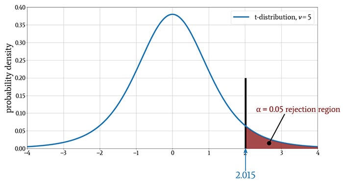
A significance level of (for example) 0.05 indicates that in order to reject the null hypothesis, the t-value must be in the portion of the t-distribution that contains only 5% of the probability mass. In the following plot, the section shaded red contains 5% of the probability mass, and the black vertical line represents the critical value. 

The t-test thought process goes something like this:

• We assume that the null hypothesis is true, i.e., that there is no relationship between the experiment’s independent and dependent variables.
• We compare the sample mean to the population mean by computing the t-value.
• We interpret the t-value relative to the critical value, which depends on the sample size and the predetermined significance threshold.
• If the magnitude of the t-value is greater than the critical value (i.e., if it’s in the rejection region), the sample mean is so far from the population mean that the difference is probably not attributable to chance. Thus, we reject the null hypothesis, which is equivalent to asserting that the experiment has demonstrated a relationship between the independent variable and the dependent variable.

One-Tailed and Two-Tailed Tests

The previous diagram corresponds to a one-tailed t-test, meaning that the rejection region extends in only one direction. If we’re interested only in the possibility of a relationship in which the dependent variable increases, we use a one-tailed test. We also use a one-tailed test if we’re interested only in the possibility of a relationship in which the dependent variable decreases.

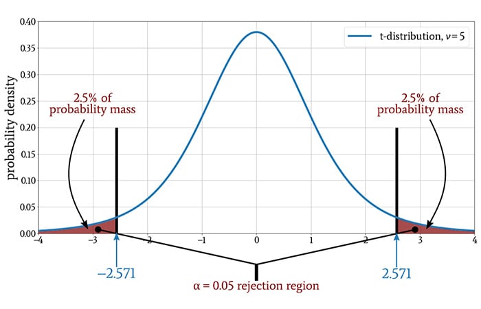
On the other hand, we might be interested in both an increase and a decrease relative to the population mean. For this, we need a two-tailed test, which splits the rejection region into a section above the mean and a section below the mean.

If we change a one-tailed test to a two-tailed test, we are splitting the same probability mass into two sections, and consequently, the critical value in the two-tailed test will be different from the critical value in the one-tailed test.

The following diagram is the two-tailed version of the t-test conditions shown in the previous diagram.

Conclusion

We’ve discussed how to calculate t-values and how to perform a One Sample t-Test, and we also covered the difference between a one-tailed test and a two-tailed test. We’ll continue this topic in the next article by applying our t-test knowledge to an example experiment.