Designing a Third-Harmonic Peaking Class F Amplifier for Maximum Efficiency

The Class F amplifier can be considered a special variant of the Class B amplifier. Unlike a Class B amplifier’s linear operation, it drives its transistor as a switch. The Class F amplifier also modifies the load network’s impedance at harmonic frequencies to adjust the voltage waveform across the transistor. Adding appropriate amounts of different harmonic components keeps the collector voltage as low as possible when the collector current is high.

In the previous article, we saw that using a third-harmonic component to produce a maximally flat waveform increases the amplifier’s efficiency from 78.5% (in a Class B amplifier) to 88.4% (in a third-harmonic peaking Class F amplifier). The term “maximally flat” refers to the fact that the derivatives of the waveform are zero at their peak values.

However, it turns out that the maximally flat waveform doesn’t produce the optimum efficiency. In this article, we’ll explore how allowing the voltage waveform to have a small amount of ripple can further increase the third-harmonic peaking amplifier’s efficiency.

 

Experimenting with the Collector Voltage Waveform

The collector voltage waveform for a third-harmonic peaking Class F amplifier can be expressed as:

$$\begin{eqnarray}v_{F} ~&=&~ V_{cc} ~-~A_1 \sin(\omega t)~-~A_3 \sin(3 \omega t) \\~&=&~V_{cc} ~-~A_1 \Big (\sin(\omega t)~+~x ~\times~ \sin(3 \omega t) \Big )\end{eqnarray}$$

Equation 1.

 

where:

A₃ is the third-harmonic component

A₁ is the fundamental component

x is the ratio of the third-harmonic component to the fundamental component (x = A₃/A₁).

For values of x less than or equal to 1/9, the waveform exhibits a single peak and a single trough. At x = 1/9, the maximally flat waveform is achieved. When x exceeds 1/9, the waveform starts to overshoot and exhibits a double peak.

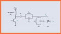
To illustrate this, Figure 1 shows the Class F collector voltage waveform (v_F) for A₁ = V_cc = 1 V and three different values of x:

• x = 0 (the red curve).
• x = 1/9 (the blue curve).
• x = 1/7 (the green curve).

Since A₁ = 1 V for all three values of x, we can also think of the waveforms in Figure 1 as representing the total collector voltage for different values of the third-harmonic component.

 

Figure 1. The total collector voltage for A₁ = V_cc = 1 V and x = 0, 1/9, and 1/7.

 

As we discussed in an earlier article, adding a third-harmonic component reduces the peak-to-peak swing of v_F. This is clearly illustrated above—the red curve, which has no third harmonic, swings from 0 to 2 V (2V_cc). By contrast, the blue curve (x = 1/9, the maximally flat waveform) swings from 0.11 V to 1.89 V.

This key characteristic of Class F operation allows us to use a fundamental frequency component that surpasses the normal swing limits set by the supply voltage. We can then increase the input power at the fundamental frequency to exploit the full potential swing, allowing us to deliver a larger power to the load.

This brings us to the green curve, which uses a third harmonic larger than that of the maximally flat waveform and appears to have an even smaller peak-to-peak swing. Figure 2 provides a zoomed-in view of the curves so that we can better see the waveform’s diminished swing.

 

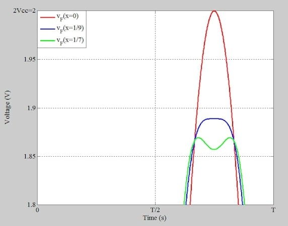
Figure 2. The zoomed-in view of the total collector voltage for A₁ = V_cc = 1 V and x = 0, 1/9, and 1/7.

 

Figures 1 and 2 suggest that a small amount of ripple in the voltage waveform might allow us to increase the power at the fundamental component. This, in turn, can enhance the amplifier’s performance by increasing the power delivered to the load.

But how much is “a small amount?” In the next section, we’ll derive the equations for a third-harmonic peaking Class F amplifier with maximum efficiency. Before diving in, however, let's conduct one last test with these waveforms by adjusting x to 1/4. The new waveform is shown in cyan in Figure 3.

 

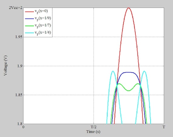
Figure 3. The zoomed-in view of the total collector voltage for A₁ = V_cc = 1 V and x = 0, 1/9, 1/7, and 1/4.

 

Once again, increasing the value of x results in a peak that surpasses that of the maximally flat waveform. This confirms that an optimal value for x must exist that maximizes the efficiency, and that this value is greater than 1/9 (the value for the maximally flat waveform).

 

Deriving the Maximum Efficiency Equation

Figure 4 shows the circuit diagram for a third-harmonic peaking Class F amplifier. To find the optimal value of x for this amplifier, we need to understand how the amplifier’s efficiency is influenced by the peak-to-peak swing of the waveform.

 

Figure 4. The third-harmonic peaking Class F amplifier.

 

Recall that the efficiency of a power amplifier is defined as:

$$\eta ~=~ \frac{P_L}{P_{cc}}$$

Equation 2.

 

where:

P_L is the average power delivered to the load

P_cc is the power drawn from the supply.

The power delivered to the load is:

$$P_L~=~\frac{1}{2}v_o i_o$$

Equation 3.

 

where v_o and i_o are the amplitudes of the voltage across the load and the current through it, respectively.

To calculate the power provided by the supply, we find the average value of the current drawn from the supply (I_c,ave) and multiply it by the supply voltage (V_cc):

$$P_{cc} ~=~ V_{cc} I_{c,ave}$$

Equation 4.

 

Substituting Equations 3 and 4 into the efficiency equation, we have:

$$\eta ~=~ \frac{1}{2} ~\times~ \frac{v_o}{V_{cc}} ~\times~ \frac{i_o}{I_{c, ave}}$$

Equation 5.

 

The conduction angle in a Class F amplifier is typically set at 180 degrees, as it would be for Class B operation. With a conduction angle of 180 degrees, we can assume that the collector current is a half-wave rectified sinusoid of amplitude I_p and period T, as shown in Figure 5.

 

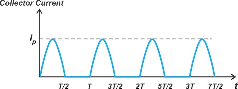
Figure 5. The collector current is a half-wave rectified sinusoid.

 

Using the Fourier series representation, the above waveform can be expressed as:

$$i_{out(t)}~=~\frac{I_p}{\pi}~+~\frac{I_p}{2} \sin (\omega_0 t)~-~\frac{2I_p}{3 \pi} \cos(2 \omega_0t)~-~\frac{2I_p}{15 \pi} \cos(4 \omega_0t)~+~...$$

Equation 6.

 

Using the above equation, we can establish relationships for the DC current drawn from the supply and the fundamental current through the load:

$$I_{c, ave} ~=~ \frac{I_p}{\pi} \quad \text{and} \quad i_o ~=~ \frac{I_p}{2}$$

Equation 7.

 

We don’t know the value of I_p in the above equations. However, we now have enough information to simplify the efficiency equation (Equation 5), leading to:

$$\eta ~=~ \frac{\pi}{4} ~\times~ \frac{v_o}{V_{cc}}$$

Equation 8.

 

We’ll learn more about the above equation in the next section.

 

Evaluating the Efficiency Equation

Equation 8 establishes a simple relationship between the output voltage swing and the efficiency of the amplifier. The underlying assumption of this equation is that the conduction angle is 180 degrees, which means that the collector voltage waveform is a half-wave rectified sinusoid. The equation should therefore be valid for both a Class B amplifier and a maximally flat Class F amplifier.

Let’s check the truth of this statement. The maximum amplitude of the output swing in a Class B amplifier is v_o = V_cc. Applying this to Equation 8, the maximum efficiency of the Class B amplifier works out to its widely known value of π/4, as calculated below:

$$\eta ~=~ \frac{\pi}{4} ~\times~ \frac{v_o}{V_{cc}}~=~\frac{\pi}{4}~=~78.5 \ \%$$

Equation 9.

 

For a maximally flat Class F amplifier, the parameters of the collector voltage equation (Equation 1) are x = 1/9 and A₁ = 9V_cc/8. Therefore, the efficiency equation simplifies to:

$$\eta ~=~ \frac{\pi}{4} ~\times~ \frac{v_o}{V_{cc}}~=~\frac{\pi}{4} ~\times~ \frac{9}{8}~=~88.4 \ \%$$

Equation 10.

 

which is consistent with the analysis provided in the preceding article.

 

Maximum Efficiency of the Third-Harmonic Peaking Class F Amplifier

Now that we’ve confirmed the validity of our new efficiency equation, let’s put it to use. Equation 8 shows that the maximum efficiency occurs when the ratio of the output voltage swing to the supply voltage (v_o/V_cc) is also maximized. The output swing is determined by the amplitude of the fundamental component (A₁). Therefore, for a given supply voltage, we need to find the value of the third harmonic (A₃) that allows us to maximize A₁.

We’ll bypass the detailed mathematical analysis here and go straight to outlining the conditions for maximum efficiency. The efficiency of the third-harmonic peaking amplifier is maximized when:

$$x~=~ \frac{1}{6}~\approx~ 0.1667$$

Equation 11.

 

where x = A₃/A₁. Under this condition, and equating the minimum collector voltage to zero (v_F = 0), we obtain the absolute values of A₁ and A₃ in terms of the supply voltage:

$$A_1 ~=~ \frac{2}{\sqrt{3}} ~\times~ V_{cc}$$

Equation 12.

 

and:

$$A_3 ~=~ \frac{1}{3 \sqrt{3}} ~\times~ V_{cc}$$

Equation 13.

 

Figure 6 plots the optimally efficient voltage waveform. The waveform for x = 0 is also included for purposes of comparison.

 

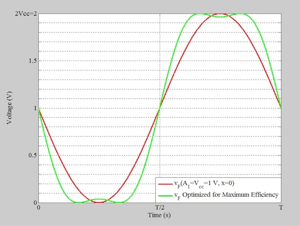
Figure 6. The green curve shows the collector voltage waveform for the maximum-efficiency amplifier (A₁ = V_cc = 1 V, x = 1/6).

 

Equation 12 established a relationship between A₁ and V_cc for a maximum-efficiency third-harmonic peaking amplifier. Combining this equation with the efficiency equation we derived earlier (Equation 8), we can now determine the achievable efficiency:

$$\eta ~=~ \frac{\pi}{4} ~\times~ \frac{v_o}{V_{cc}}~=~ \frac{\pi}{4} ~\times~ \frac{2}{\sqrt{3}}~=~90.7 \ \%$$

Equation 14.

 

With voltage ripple added, the third-harmonic peaking Class F amplifier has a maximum efficiency of 90.7%.

 

Example: Designing a Third-Harmonic Peaking Amplifier For Maximum Efficiency

A Class F amplifier with third-harmonic peaking is designed for maximum efficiency. For an output power of P_L = 10 W and a supply voltage of V_cc = 12 V, determine the following:

• The load resistance (R_L).
• The maximum current and voltage that the transistor must tolerate.

We can use the equation for the amplifier’s output power to find the load resistance (R_L). The output power can be found by:

$$P_L~=~ \frac{v_{o, rms}^2}{R_L}~=~ \frac{1}{2}\frac{ A_1^2}{R_L} \quad \rightarrow \quad P_L ~=~ \frac{2}{3} ~\times~ \frac{V_{cc}^2}{R_L}$$

Equation 15.

 

In the above equation, we’ve substituted the value of A₁ from Equation 12. With P_L = 10 W and V_cc = 12 V, we obtain R_L = 9.6 Ω.

The maximum collector voltage is 2V_cc , which in this case = 24 V. To determine the maximum collector current (I_p), we note that the amplitude of the fundamental collector current is I_p/2. This current flows into the load (R_L) and produces a fundamental voltage amplitude of \(A_1 ~=~ (\frac{2} {\sqrt3})V_{cc}\). Therefore, we have:

$$\frac{I_p}{2} ~\times~ R_L ~=~\frac{2}{\sqrt{3}} V_{cc} \quad \rightarrow \quad I_p ~=~ \frac{4}{\sqrt{3}} ~\times~ \frac{V_{cc}}{R_L}$$

Equation 16.

 

Substituting our example values into this equation, we obtain I_p = 2.89 A.

 

Wrapping Up

As we’ve now seen, the maximum theoretical efficiency of a third-harmonic peaking Class F amplifier is η = 90.7%. In the next article, we’ll learn about a different Class F amplifier configuration, the transmission-line peaking Class F amplifier, that can improve the efficiency even further.

 

This article is Part 23 of a series on power amplifier classes. A complete list of articles in this series is provided below.

 

Classes A through C:

Class D:

Class E:

Class F and Inverse Class F:

 

All images used courtesy of Steve Arar