Harmonic Suppression in Low-Q Class E Amplifiers

In this article, we examine the filtering requirements of Class E power amplifiers with less-than-ideal Q-factors.

Technical Article October 23, 2024 by Dr. Steve Arar

The previous article in this series explored the idealized operation of a Class E amplifier and derived its design equations. As we discussed near the end of the article, these equations rely on the load network’s quality factor (Q) being high enough to ensure a sinusoidal output current at the switching frequency. Otherwise, the basic design equations may not produce the zero-voltage and zero-derivative switching conditions necessary for optimum performance.

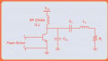
The practical range of Q is from 3 to 10, which isn’t high enough to prevent harmonic currents from flowing into the load. Figure 1 shows a basic Class E amplifier—to provide the required degree of harmonic suppression, we need to insert a filter between its series resonant circuit and its load.

Schematic of a basic Class E amplifier.

Figure 1. Schematic of a basic Class E amplifier. Image used courtesy of Steve Arar

In this article, we’ll learn how to determine the necessary filter attenuation for achieving the desired harmonic suppression. Before we reach those calculations, however, we need to discuss the frequency content of the amplifier’s switch waveforms. We’ll start with the switch voltage.

Frequency Content of the Switch Voltage

Figure 2 shows the typical switch waveforms for a Class-E driven transistor.

Typical switch current and voltage waveforms for a Class E amplifier.

Figure 2. Typical switch current (top) and voltage (bottom) waveforms in a Class E amplifier. Image used courtesy of Steve Arar

The classic paper “Idealized Operation of the Class E Tuned Power Amplifier” by F. Raab calculates the spectrum of the switch voltage waveform (V_sw in the above figure). In this paper, Dr. Raab represents the n-th harmonic voltage component (V_n) as:

$$V_n~=~c_n \sin(n \omega t ~+~ \phi_n)$$

Equation 1.

where:

n = the harmonic number

c_n = the amplitude of the n-th harmonic

⍵ = the frequency (in rad/s)

t = time

ϕ_n = the phase angle of the n-th harmonic.

His analysis leads to the spectrum shown in Figure 3. Note that the values of c_n in this figure are normalized to the supply voltage. Put a different way, it assumes V_cc = 1.

The spectrum of voltage across a Class-E driven switch.

Figure 3. The spectrum of the voltage across a Class-E driven switch. Image used courtesy of F. Raab

In an optimum Class E amplifier, the amplitudes of the harmonic components decrease with 1/n². The amplitudes of the first five harmonic components are given in Table 1 along with the gain in decibels.

Table 1. The amplitudes of an optimum Class E amplifier’s first five harmonic voltage components. Data used courtesy of N. O. Sokal

n	1	2	3	4	5
c_n	1.6390	0.8477	0.2222	0.1432	0.0800
c_n in dB	0	–5.73	–17.36	–21.17	–26.23

As an aside, the harmonic components of a mistuned amplifier reduce at a slower rate of 1/n. This is illustrated by the dotted line in Figure 3.

Frequency Content of the Load Current

To obtain the n-th harmonic current, we divide the amplitude of the corresponding harmonic voltage (c_n) by the input impedance of the load network at that frequency (Z_n):

$$i_n ~=~ \frac{c_n}{Z_n}$$

Equation 2.

Based on the above equation, the amplitude of the n-th harmonic current normalized to the fundamental harmonic current is:

$$\frac{i_n}{i_1} ~=~ \frac{c_n}{c_1} ~\times~ \frac{Z_1}{Z_n}$$

Equation 3.

The input impedance of the load network at a given harmonic frequency can be approximated by the reactance of the series resonant circuit at that frequency. For the amplifier in Figure 1, this corresponds to the series combination of L₀ and C₀. We therefore have:

$$|Z_n| ~=~ L_0 n \omega ~-~ \frac{1}{C_0 n \omega}$$

Equation 4.

In an optimum Class E amplifier, the values of L₀ and C₀ are given by:

$$L_{0} ~=~ \frac{Q R_L}{\omega}$$

Equation 5.

and:

$$C_{0} ~=~C_{sh} ~\times~ \frac{5.447}{Q} ~\times~ \big ( 1~+~ \frac{1.42}{Q~-~2.08} \big )$$

Equation 6.

where R_L is the load resistance and C_sh is the shunt capacitance. To find C_sh, we use the following equation:

$$C_{sh} ~=~ \frac{0.1836}{\omega R_L}$$

Equation 7.

Substituting Equations 5, 6, and 7 into Equation 4 produces an expression for Z₁/Z_n, the normalized harmonic impedance:

$$\frac{Z_1}{Z_n} ~=~ \frac{1.42}{nQ} ~\times~ \frac{1}{(1~-~1/n^2)~-~\big ( 0.66~-~2.08/n^2 \big )/Q}$$

Equation 8.

In this equation, Z₁/Z_n is a function only of the harmonic number (n) and the Q-factor. The equation shows that Z_n increases roughly in proportion to n, at least when n and Q are relatively large. For a more detailed discussion of Equations 4 through 8, please refer to the paper “Harmonic Output of Class-E RF Power Amplifiers and Load Coupling Network Design” by N. O. Sokal and F. Raab.

Moving on, Table 2 shows the ratio Z₁/Z_n for the first five harmonic frequencies with a Q-factor of 5.

Table 2. The first five normalized harmonic impedances for Q = 5.

n	1	2	3	4	5
Z₁/Z_n	1	0.1967	0.1179	0.0854	0.0672

Substituting the values from Tables 1 and 2 into Equation 3, we obtain the harmonic components of the load current (Table 3).

Table 3. Harmonic currents flowing into the load for Q = 5.

n	1	2	3	4	5
i_n/i₁	1	0.1017	0.0160	0.0075	0.0033
i_n/i₁ in dB	0	–19.85	–35.92	–42.50	–49.63

For an optimum Class E amplifier with Q = 5, the second and third harmonics of the load current are 19.85 dB and 35.92 dB lower than the fundamental component, respectively. Acceptable harmonic levels for a radio transmitter would be in the range of 60 dB below the carrier signal. To achieve these levels, we need to implement extra filtering before the load. This is illustrated in Figure 4.

Schematic of a Class E amplifier with an added output filter.

Figure 4. Class E amplifier with an added filter. Image used courtesy of Steve Arar

But how much extra filtering? In the next section, we’ll determine how much attenuation the filter must provide to suppress the harmonics to an acceptable level.

Determining the Required Filter Response

Our goal is to keep all harmonic components of the load current (i_out) at least 60 dB lower than the fundamental component. Converted from decibels, this means that the harmonic components at the load should be lower than the fundamental component by a factor of at least 1,000.

Let’s start with the second harmonic. Table 3 shows that, at the input of the filter, the second harmonic is lower than the fundamental by a factor of 0.1017:

$$i_{in,2} ~=~ 0.1017 ~\times~ i_{in,1}$$

Equation 9.

where i_in,₂ and i_in,₁ denote, respectively, the second and fundamental harmonic of the current flowing into the filter.

At the output of the filter, we want the second current harmonic to be at least 1,000 times lower than the fundamental current:

$$i_{out,2} ~=~ \frac{1}{1000} ~\times~ i_{out,1}$$

Equation 10.

To suppress the harmonic component to the desired level, the filter should provide more attenuation at the second harmonic than at the first. If the filter’s current gain at the second harmonic relative to its gain at the fundamental frequency is A₂, we should have:

$$0.1017 ~\times~ A_2 ~=~ \frac{1}{1000} ~~\rightarrow ~~A_2 ~=~ 0.0098$$

Equation 11.

We can also perform these calculations in decibels. At the input of the filter, the second harmonic is lower than the fundamental by |20log(0.1017)| = 19.85 dB. At the output, the second harmonic must be 60 dB lower than the fundamental. Therefore, the filter attenuation at the second harmonic must be at least 40.15 dB greater than that at the fundamental frequency. In linear terms, –40.15 dB corresponds to an attenuation factor of 0.0098, which is consistent with Equation 11.

We can use a similar procedure to find the required attenuation at other harmonic frequencies. To do so, we use the decibel values of the current ratios (i_n/i₁) in Table 3. These values are shown, along with the filter current gain (A_n), in Table 4.

Table 4. The required filter attenuation to keep output harmonics 60 dB lower than the fundamental for Q = 5.

n	1	2	3	4	5
i_n/i₁ in dB	0	–19.85	–35.92	–42.5	–49.63
A_n in dB	0	–40.15	–24.08	–17.5	–10.37

Note that the required filter attenuation is lower for higher harmonics. This is because the series resonant circuit of the Class E configuration presents a larger impedance—and, consequently, a larger attenuation—as we move to higher frequencies. The attenuation required of the external filter is therefore lower.

Wrapping Up

A practical Class E amplifier will likely have a Q-factor of between 3 and 10. When that’s the case, we need to include an output filter in our design to prevent excessive harmonic currents from flowing into the load. In this article, we determined the required external filtering for a design with a Q-factor of 5.

Note that harmonic suppression isn’t the only requirement we need to think about. Other considerations, such as impedance matching and bandwidth, may impose additional requirements on the filter design. For those who want more information, my references for this article are listed below: