L-type Matching Network Basics—Examining L Network Frequency Response and Bandwidth

Two-element networks, known as L-sections or L-networks, can be used to transform one impedance to another. Not only that, but they are also easy to design and can be quite practical.

In this article, we’ll take a look at the frequency response of these circuits and learn about a convenient solution to estimate their bandwidth. We’ll also see that the major limitation of L-networks is their fixed bandwidth, which leads us to more complicated matching networks, such as T networks.

 

One Impedance Matching Problem, Many Solutions

For a given impedance matching problem, there are several different solutions. Let's consider designing a two-element lumped matching network; one can find at least two L-sections for any given load and input impedances. Depending on the impedance values, it is also possible to have a total of four different L-type solutions. As an example, consider transforming the impedance Z₁ = 10 + j30 Ω to the origin of the Smith chart. With a normalizing impedance of Z₀ = 50 Ω, we obtain the matching solutions shown below in Figure 1.

 

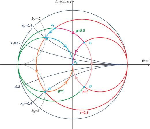
Figure 1. Example Smith chart showing matching solutions.

 

Using the intersection points A, B, C, and D, we can have four different paths from z₁ to z₂. You can use a complete ZY Smith chart to find the reactance (x) and susceptance (b) of the intersection points. These values are listed in Table 1.

 

Table 1. ZY Smith chart intersection points, reactance, and susceptance values.

Intersection Point	Reactance (x)	Susceptance (b)
A	0.4	-2
B	-0.4	2
C	1	-0.5
D	-1	0.5

 

Using these values, we obtain the following L-sections for this impedance-matching problem (Figure 2).

 

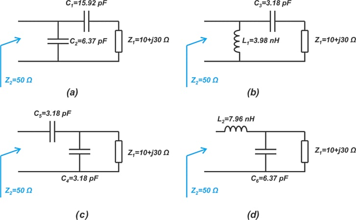
Figure 2. L-sections for our impedance-matching example problem.

 

The L-sections in Figure 2 (a), (b), (c), and (d), respectively, correspond to paths going from z₁ to z₂ through the points A, B, C, and D on the Smith chart. The component values are calculated at an operating frequency of 1 GHz. The question that arises at this point is, how do we choose the appropriate matching network from these available options? To answer this question, let’s first look at the frequency response of these matching networks.

 

L-Section Frequency Response

Let’s assume that the load impedance Z₁ = 10 + j30 Ω in the above example is a series RL circuit. At 1 GHz, we have R = 10 Ω and L = 4.77 nH. The input reflection coefficient of our L-sections is shown in Figure 3 below.

 

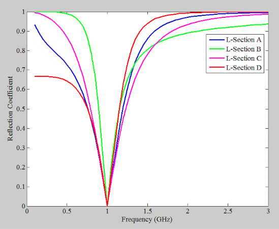
Figure 3. Graph showing the input reflection coefficient of our L-sections.

 

As can be seen, the reflection coefficient is almost zero at 1 GHz, meaning that all of these matching circuits provide an input impedance of about 50 Ω at a narrow band around 1 GHz (no big surprise!). Next, we'll look at the input-output transfer function of each circuit. Figure 4 shows how we’ve defined the input and output signals for this simulation.

 

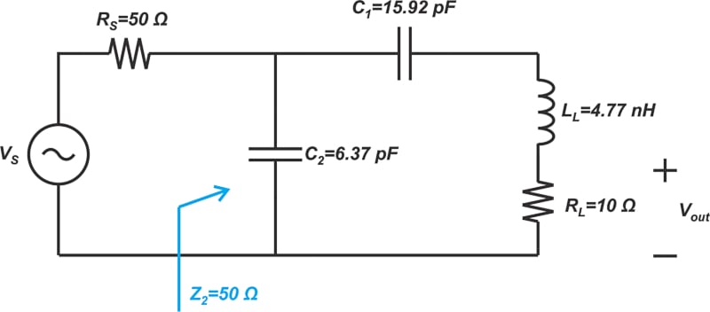
Figure 4. Example diagram of the input and output signals from the transfer function simulation. 

 

A voltage source with a source resistance of 50 Ω is applied to the input of the matching network. The output signal is the voltage across the resistive part of the load. The simulated transfer function of the above L-networks in decibels \(20log ( \frac{V_{out}}{V_S})\) is shown in Figure 5. 

 

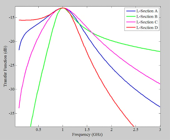
Figure 5. A graph showing the transfer function vs frequency for the L-network sections.

 

The L-sections in Figure 2(a) and (c), each consisting of two capacitors, pass a narrow band around 1 GHz and reject frequencies below and above this center frequency by almost the same amount. These structures have a bandpass response ( → assuming that the load has a resistive part!). The L-network in Figure 2(b) blocks DC and severely attenuates frequencies below 1 GHz. In this case, we have a highpass frequency response.

Finally, the L-section in Figure 2(d) is a lowpass circuit; it passes DC and rejects higher frequencies. As the above example shows, the frequency response of an L-section can be lowpass, highpass, or bandpass. Note that even for the lowpass and highpass cases, a gain peaking occurs at the frequency at which the impedance match is provided. In general, there are eight possible arrangements of L-type matching networks, as shown in Figure 6.

 

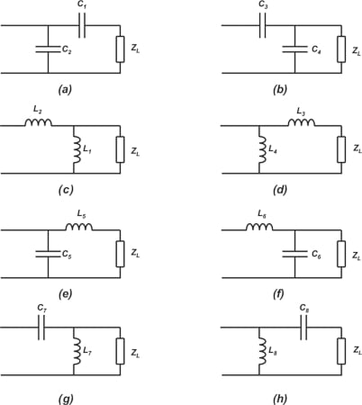
Figure 6. Eight potential L-type matching network arrangements.

 

The L-sections in Figure 6 (a), (b), (c), and (d), each consisting of either two capacitors or two inductors, have a bandpass response. Figures 6(e) and (f) show lowpass L-type matching networks, while Figures 6(g) and (h) are highpass structures.

 

Choosing the Right L-section

The actual choice between different types of L-sections (and matching networks in general) depends on the application. For example, the highpass response of the L-section in Figure 5(b) provides AC coupling (or DC isolation) that might be required in many applications. On the other hand, some applications need a lowpass matching network to provide DC feed-through between the input and output terminations.

Additionally, depending on the parasitic reactive components of the load and source impedances, we might prefer to use a particular type of L-section network. As an example, assume that the load has some parasitic parallel capacitance. In this case, it might be possible to use an L-section with a parallel capacitor on the load side to absorb the undesired capacitance of the load into the impedance-matching network. Another important factor is the bandwidth of the matching network, but we’ll get into it in another section.

 

Estimating L-section Bandwidth

The bandwidth of an L-section can be relatively wide. For example, with the responses shown in Figure 5, the bandwidth changes from about 480 MHz (L-section D) to 790 MHz (L-section A). The quality factor concept Q_L, defined below, is normally used to parameterize the bandwidth of L-sections:

 

\[Q_L=\frac{f_0}{BW}\]

Equation 1.

 

In the above equation, f₀ is the frequency where the match occurs, and BW is the -3dB bandwidth of the frequency response. For example, with the blue curve in Figure 5, we have f₀ = 1 GHz and BW = 1.32 GHz - 0.53 GHz = 790 MHz, leading to Q_L = 1.27. There is a convenient method of estimating the quality factor of an L-section. To this end, we first need to define the nodal quality factor that is obtained from the equivalent impedance or admittance of different nodes of the matching circuit. If the equivalent impedance of a node is Z = R + jX, the node quality factor is defined as:  

 

\[Q_n=\frac{|X|}{R}\]

Equation 2.

 

The node quality factor can also be obtained from the admittance of the node. If the equivalent admittance of a node is Y = G + jB, we have:

 

\[Q_n=\frac{|B|}{G}\]

Equation 3.

 

At each node of the L-type matching network, we can use either Equation 1 or 2 to find the quality factor of that node (both equations produce the same value). Each node in the circuit has its own nodal Q. If the maximum value of the circuit’s nodal quality factor is Q_n, then we can use the following equation to estimate the quality factor of an L-section:

 

\[Q_L=\frac{Q_n}{2}\]

Equation 4.

 

Note that this equation is only an approximation of the actual Q_L. Let’s look at an example.

 

Estimating L-section Bandwidth Example

Continuing with the matching problem in Figure 1, we observe that the maximum nodal Q occurs at point z₁ (corresponding to Z₁ = 10 + j30):

 

\[Q_n=\frac{|X|}{R}=\frac{30}{10}=3\]

 

You can verify that at points A and C, we have a smaller nodal Q of 2 and 1, respectively. With Q_n = 3, Equation 4 leads to Q_L = 1.5. By substituting Q_n = 1.5 and f₀ = 1 GHz into Equation 1, the bandwidth is estimated to be BW = 667 MHz. The actual bandwidth changes from about 480 MHz (L-section D) to 790 MHz (L-section A). Considering the simplicity of the approximation equations, the estimated bandwidth is in reasonable agreement with the actual value.

 

The L Network Fixed Bandwidth Limitation and a T Network Introduction

As mentioned, L-sections are simple to design and quite practical. However, they have one major disadvantage; their bandwidth is determined by the input and output impedance. To better understand this, consider transforming z_Load = 0.2 to the center of the Smith chart, as illustrated in Figure 7.

 

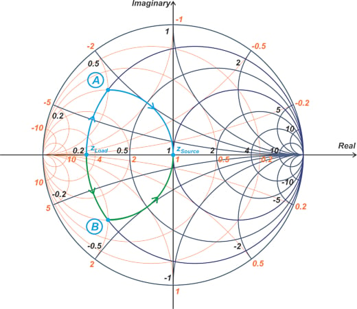
Figure 7. Example Smith chart with z_Load = 0.2.

 

The intermediate impedances are the intersection points of the r = 0.2 and g = 1 circle. As you can see, the intersection points are determined by the source and load impedances. Therefore, the nodal Q and, consequently, the bandwidth of the matching network are fixed. In this example, Q_n is 2. If our application needs a higher or lower Q, we can use two intermediate impedances (rather than a single intermediate point) going from z_Load to z_Source. As an example, assume that we need to have a maximum Q_n of 5. One solution for this case uses intermediate points C and D, as shown in Figure 8.

 

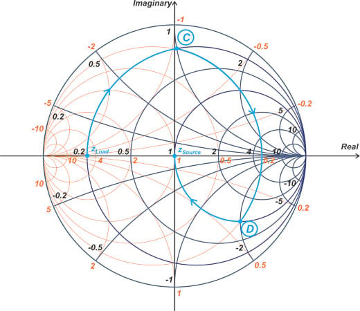
Figure 8. Smith chart showing intermediate points C and D.

 

We first move along the r = 0.2 constant-resistance circle to point C which has a normalized impedance of 0.2 + j. Next, we move along the g = 0.2 constant-conductance circle to point D, which has a normalized impedance of 1 - j2. Finally, we follow the r = 1 constant-resistance circle to arrive at the center of the Smith chart. In this case, the maximum nodal Q occurs at point C, producing Q_n = 5. Having two intermediate points is equivalent to having a three-element matching network.

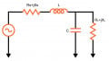
In the above example, the first motion from z_Load to C as well as the third motion from D to z_Source are along constant-resistance circles. These correspond to adding series components. The second motion, however, is along a constant-conductance circle, requiring a parallel component. Therefore, the matching network should have a “T network” arrangement (Figure 9).

  

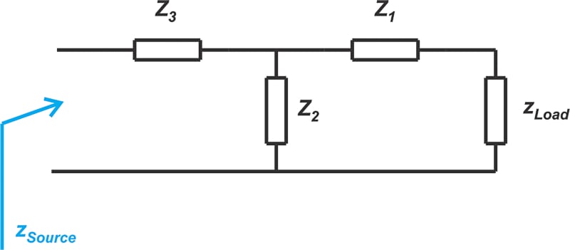
Figure 9. Diagram showing a T network.

 

The addition of a third element allows us to have control over the maximum nodal Q of the circuit. Unlike an L-type network, it is not easy to find a simple relationship between the loaded quality factor (Q_L) of the T network and the Q of the circuit nodes. However, it is obvious that a high value of Q_n leads to a higher value of Q_L. In the next article in this series, we’ll continue this discussion and learn about other impedance-matching networks.

 

Summarizing L Network Basics

• L-sections are easy to design but quite practical.
• For a given impedance matching problem, there might be several different L-sections as well as other more complicated matching networks, such as T-type solutions.
• The choice of the matching network is affected by several considerations, such as DC biasing, the type of frequency response (lowpass or highpass), bandwidth, and ease of implementation, to name a few.
• If we need to have control over the bandwidth, we might need to use more complicated matching networks, such as a T network rather than an L-section.

 

---

 

To see a complete list of my articles, please visit this page.