Technical Article

Linear Filtering Based on the Discrete Fourier Transform

October 19, 2017 by Dr. Steve Arar

The DFT provides an efficient way to calculate the time-domain convolution of two signals.

One of the most important applications of the Discrete Fourier Transform (DFT) is calculating the time-domain convolution of signals. This can be achieved by multiplying the DFT representation of the two signals and then calculating the inverse DFT of the result.

You may doubt the efficiency of this method because we are replacing the convolution operation with two DFTs, one multiplication, and an inverse DFT operation. However, since there are efficient methods of calculating the DFT, collectively called the Fast Fourier Transform (FFT), we can gain significant computational saving by using the DFT to perform the time-domain convolution.

Note that the difference equation of a Finite Impulse Response (FIR) filter, repeated below for the convenience, is actually calculating the convolution of the input sequence, $$x(n)$$, with the filter coefficients $$b_k$$:

$$y(n)=\sum_{k=0}^{M-1}b_{k}x(n-k)$$

Hence, the DFT-based method can be particularly helpful in implementing an FIR filter. For a filter longer than nearly 64 taps, the DFT-based method would be computationally more efficient than the direct- or cascade-form structures (see the last section of chapter 18 of this book).

In this article, we will briefly review the linear convolution. Then, after pointing out some observations about the linear convolution and the DFT, we will see how the DFT can be used to perform the linear convolution. We will also see that the inverse DFT of the product of the DFT of two signals corresponds to a time-domain operation called the circular convolution.

Linear Convolution

The linear convolution of two signals $$x(n)$$ and $$h(n)$$ is given by

$$y(n)=\sum_{k=-\infty}^{+\infty}x(k)h(n-k)$$

Equation 1

This is the fundamental equation that allows us to analyze the response of a linear time-invariant system to an arbitrary input sequence, $$x(n)$$, only having the impulse response of the system $$h(n)$$.

As an example, assume that $$x(n)$$ and $$h(n)$$ are as shown in Figure 1 and 2, respectively. The convolution of these two signals will be as shown in Figure 3. You can use the MATLAB function conv() to verify this result without getting involved in the mathematics.

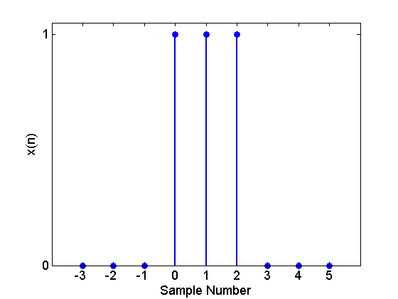
Figure 1

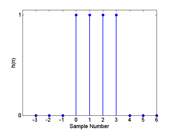
Figure 2

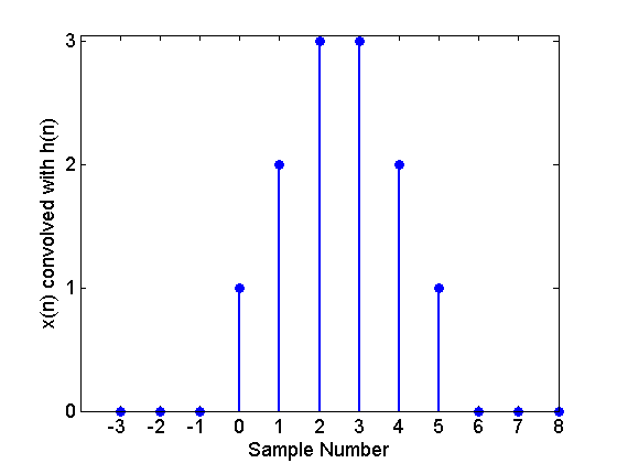
Figure 3. The convolution of $$x(n)$$ with $$h(n)$$.

Assume that $$x(n)=0$$ when $$n<0$$ or $$n \geq L$$, besides, $$h(n)=0$$ for $$n<0$$ or $$n \geq K$$. Let’s examine the convolution sum of Equation 1 under these conditions and see what values of $$n$$ will give $$y(n)=0$$. This will help us determine the maximum number of nonzero values that a convolution sum may have.

$$y(n)$$ in Equation 1 will be zero if $$x(k)$$ or $$h(n-k)$$ are zero for a given $$n$$. $$x(k)$$ can be nonzero only if $$0 \leq k \leq L-1$$. For these values of $$k$$, we need $$h(n-k)$$ to be zero to make $$y(n)=0$$. This would happen if $$n-k<0$$ or $$n-k>K-1$$. The condition $$n-k<0$$ along with the range of $$k$$, i.e. $$0 \leq k \leq L-1$$, gives $$y(n)=0$$ for $$n \leq -1$$. Moreover, the condition $$n>K-1+k$$ along with $$0 \leq k \leq L-1$$ gives $$y(n)=0$$ for $$n \geq K+L-1$$. This is our first observation which is summarized below:

Observation 1:

Assume that $$x(n)=0$$ when $$n<0$$ or $$n \geq L$$, besides, $$h(n)=0$$ for $$n<0$$ or $$n \geq K$$. Then $$y(n)=x(n) \star h(n)$$ can be nonzero only for $$0 \leq n \leq K+L-2$$. Sometimes we put it this way: if $$x(n)$$ and $$h(n)$$ are two signals of length $$L$$ and $$K$$, respectively, then, the convolution of these two signals will be of length $$L+K-1$$.

The signals illustrated by Figure 1, 2, and 3 are an example of this observation. In this case, we have $$L=3$$ and $$K=4$$. The convolution of these two signals is a signal with $$L+K-1=3+4-1=6$$ nonzero values.

Time-domain Convolution Using the Fourier Analysis

We can use the Fourier analysis to calculate the time-domain convolution in the frequency domain. Expressed mathematically, we have

$$F \{ x(n) \star h(n) \}=X(\omega)H(\omega)$$

Equation 2

where $$F \{ . \}$$ denotes the Discrete-Time Fourier Transform (DTFT) operation. And, $$X(\omega)$$ and $$H(\omega)$$ are the DTFTs of $$x(n)$$ and $$h(n)$$, respectively. From a theory point of view, Equation 2 is a very important result; however, we cannot use this property on a digital computer because the DTFT of a sequence is a continuous function of $$\omega$$. The obvious solution will be using samples of the DTFT, which is called the DFT.

To apply the DFT, we must have finite-duration signals. Can we use the finite-duration signals $$x_1(n)$$ and $$h_1(n)$$ in Figure 4 and 5 to represent $$x(n)$$ and $$h(n)$$ of Figure 1 and 2, respectively?

To answer this question we can compare the DTFT of infinitely-long sequences with the DFT of the finite-duration signals. If the DFT still gives the samples of the DTFT, then our finite-duration representation is valid. We can easily compare the DTFT of $$x(n)$$, given by

$$X(\omega)=\sum\limits_{n=-\infty}^{+\infty}{x(n){{e}^{-j \omega n}}}=1+e^{-j\omega}+e^{-j2\omega}$$

Equation 3

with the three-point DFT of $$x_1(n)$$ which is

$$X_{1}(k)=\sum\limits_{n=0}^{2}{x(n){{e}^{-j\tfrac{2\pi }{3}kn}}}=1+{e}^{-j\tfrac{2\pi }{3}k \times 1}+{e}^{-j\tfrac{2\pi }{3}k\times 2}$$

Equation 4

Obviously, the summations of Equation 3 and 4 are equal for $$\omega =\tfrac{2\pi}{3}k$$, $$k=0, \; 1, \; 2$$. Since the DFT of the finite-duration sequence gives samples of the DTFT of $$x(n)$$, we can use $$x_1(n)$$ when applying the DFT.

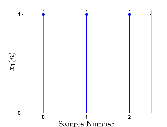
Figure 4. The finite-duration version of $$x(n)$$.

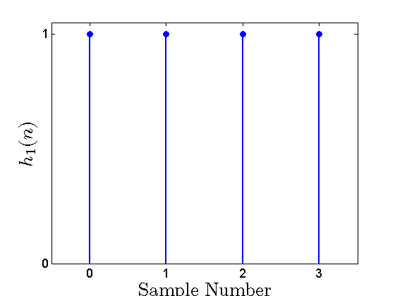
Figure 5. The finite-duration version of $$h(n)$$.

To use the samples of the DTFTs in Equation 2, we need to multiply a given sample of $$X(\omega)$$ at frequency $$\omega_i$$ by the sample of $$H(\omega)$$ at the same frequency, i.e. $$H(\omega_i)$$. Hence, the DFT of $$x(n)$$ should give the same frequency points as the DFT of $$h(n)$$.

Since the frequency points of an N-point DFT are the normalized frequencies $$\tfrac{2\pi}{N}k$$, for $$k=0, 1, \dots , N-1$$, the length of the DFT must be the same for both $$x(n)$$ and $$h(n)$$. However, as shown in Figure 4 and 5, the two signals $$x_1(n)$$ and $$h_1(n)$$ are not necessarily of the same length. To make the two signals of the same length, we can insert zeros at the end of the shorter signal. This is called zero-padding.

We will represent the zero-padded version of $$x_1(n)$$ with $$x_2(n)$$ which is shown in the following figure.

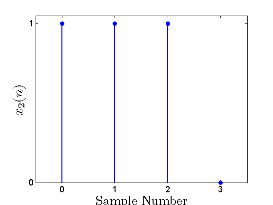
Figure 6. The zero-padded version of $$x_1(n)$$.

Comparing the DFT of $$x_2(n)$$ with the DTFT of $$x(n)$$, we can easily verify that the DFT of the zero-padded signal gives four samples of the DTFT in contrast to the DFT of $$x_1(n)$$ which gives only three samples. Hence, the zero-padding technique increases the number of samples that we get from a particular DTFT. Some textbooks put it this way: zero-padding increases the computational resolution of the DFT.

Observation 2:

To use the samples of the DTFTs in Equation 2, we need to multiply a given sample of $$X(\omega)$$ at frequency $$\omega_i$$ by the sample of $$H(\omega)$$ at the same frequency, i.e. $$H(\omega_i)$$. Hence, the length of the DFT must be the same for both $$x(n)$$ and $$h(n)$$. If the two signals are not of the same length, we can insert adequate zeros at the end of the shorter signal.

In the above example, we inserted a single zero and achieved two signals of length four. Now, can we calculate the four-point DFT of $$h_1(n)$$ and $$x_2(n)$$ and multiply them to find the DFT of the convolution $$h_1(n) \star x_2(n)$$?

To answer this question, we need to review an important property of the DFT analysis: assume that we calculate the N-point DFT of a finite-duration sequence such as $$x(n)$$ and achieve $$X(k)$$. While, we obtain $$X(k)$$ as a representation for the finite-duration sequence $$x(n)$$, it can be shown that the time-domain signal corresponding to $$X(k)$$ is actually a periodic signal with period $$N$$. This periodic signal can be achieved by repeating the values of the finite-duration sequence $$x(n)$$ with period $$N$$. In other words, one period of this periodic signal produces the same values that $$x(n)$$ does. (Please see this article for a detailed discussion of the periodic nature of the DFT.)

Based on this property of the DFT, we know that a four-point DFT corresponds to a time-domain periodic signal with period four. Hence, if we multiply the four-point DFT of $$h_1(n)$$ and $$x_2(n)$$, the result, $$H_1(k)X_2(k)$$, will correspond to a time-domain periodic signal with period four. We were initially expecting $$H_1(k)X_2(k)$$ to be the DFT of $$h_1(n)x_2(n)$$; however, this is not possible because $$h_1(n) \star x_2(n)$$ is a signal of length $$L+K-1=3+4-1=6$$ and, generally, it cannot be represented with a periodic signal with period four.

As you may have guessed, we need to calculate the N-point DFT of $$h_1(n)$$ and $$x_2(n)$$ for $$N \geq L+K-1=6$$ to be able to obtain the convolution of $$h_1(n) \star x_2(n)$$ by applying the inverse DFT to the product of DFTs of $$h_1(n)$$ and $$x_2(n)$$. Clearly, we will have to insert enough zeros to make both $$x_2(n)$$ and $$h_1(n)$$ of length $$N$$.

Observation 3:

If $$x(n)$$ and $$h(n)$$ are two signals of length $$L$$ and $$K$$, respectively, then, the convolution of these two signals will be of length $$L+K-1$$. Considering the periodic nature of the DFT analysis, DFTs longer than $$L+K-1$$ are required to calculate the time-domain convolution, $$x(n) \star h(n)$$, with the DFT method.

Please note that we have not given the proof of the above statement, we are only showing that the DFT-based method to calculate the time-domain convolution requires DFTs longer than $$L+K-1$$. You can see the proof of this statement in the textbooks (see Section 3.4.1 of this book).

In fact, the inverse DFT of the product of DFTs of two signals corresponds to an operation called circular convolution in the time domain. In the rest of the article, we will briefly review the circular convolution.

Circular Convolution

Assume that $$y_1(n)$$ and $$y_2(n)$$ are two finite duration signals of length $$N$$. Then the circular convolution of these two signals is defined as

$$y_{3}(n)=\sum_{n=0}^{N-1}y_{1}(n)y_{2}\big ( (m-n) \; modulo \; N \big)$$

Equation 4

where $$m=0, 1, \dots , N-1$$ and $$(m-n) \; modulo \; N$$ represents the remainder of division of $$(m-n)$$ by $$N$$.

Assume that the N-point DFT of $$y_1(n)$$ and $$y_2(n)$$ are $$Y_1(k)$$ and $$Y_2(k)$$, respectively. Then it can be shown that $$Y_1(k)Y_2(k)$$ is the N-point DFT of the circular convolution of $$y_1(n)$$ and $$y_2(n)$$.

Now we can restate our findings based on the circular convolution: Assume that $$x(n)$$ and $$h(n)$$ are of length $$L$$ and $$K$$, respectively. Applying the N-point DFT to these signals, we obtain $$X(k)$$ and $$H(k)$$. The product $$X(k)H(k)$$ is the N-point DFT of the circular convolution of $$x(n)$$ with $$h(n)$$. If $$N \geq L+K-1$$, then the circular convolution will produce the values of the linear convolution. Hence, we can calculate the N-point inverse DFT of $$X(k)H(k)$$ to calculate the linear convolution of $$x(n)$$ with $$h(n)$$.

Example of the DFT-Based Convolution

Assume that $$x_1(n)$$ and $$h_1(n)$$ are as shown in Figure 4 and 5. We will apply the DFT-based method to calculate the convolution of these two signals. To avoid being involved in the mathematics, we can use the MATLAB functions fft() and ifft() to calculate the DFT and the inverse DFT. As discussed above, we need DTFs longer than $$L+K-1=6$$. The following lines of code will calculate the time-domain convolution:

x=[1 1 1 0 0 0]; %This line defines the zero-padded version of x1(n)

h=[1 1 1 1 0 0]; %This line defines the zero-padded version of h1(n)

ifft(fft(x).*fft(h)); % This line calculates the IDFT of the product of the DFTs

The result will be:

1.0000 2.0000 3.0000 3.0000 2.0000 1.0000

which matches the linear convolution which was previously illustrated in Figure 3.

Summary

One of the most important applications of the DFT is calculating the time-domain convolution of signals.
For an FIR filter longer than nearly 64 taps, the DFT-based method would be computationally more efficient than the direct- and cascade-form structures.
If $$x(n)$$ and $$h(n)$$ are two signals of length $$L$$ and $$K$$, respectively, then, the convolution of these two signals will be of length $$L+K-1$$. Considering the periodic nature of the DFT analysis, DFTs longer than $$L+K-1$$ are required to calculate a time-domain convolution with the DFT method.

Linear Filtering Based on the Discrete Fourier Transform

Join our Engineering Community! Sign-in with:

Linear Filtering Based on the Discrete Fourier Transform